Sinusoidal Steady State
Please Log In for full access to the web site.
Note that this link will take you to an external site (https://shimmer.mit.edu) to authenticate, and then you will be redirected back to this page.
(Adapted by notes from T.F. Weiss)
Introduction and Outline
Previously we showed that for systems described sets of linear differential equations, we can easily derive the system's transfer function, H(s), in the form of a rational function in s (a ratio of polynomials). That is,
We also showed that given an input u(t) = U e^{s_0t} and a set of initial conditions, the output, \mathbf{y}, is given by
where the L coefficients \{A_1,A_2,\ldots,A_l\} are determined from L initial conditions, and the \lambda_l's are the roots of the denominator polynomial, or the natural frequencies, or the poles, of H(s).
Our focus so far has been on the the roots of the denominator polynomial, the poles or natural frequencies, \lambda_1,...\lambda_L. They are important because they determine a system's stability. That is, if
then given any bounded input of the form u(t) = U e^{s_0 t}, \Re(s_0) < 0, the output y(t) remains bounded. But what happens when H(s) is used in a control system?
Suppose H(s) = \frac{n_h(s)}{d_h{s}} is used in a feedback system with a gain, K_0. Then from Black's formula, the closed-loop system function, G(s), would be
The stability of G(s) depends on its natural frequencies, which are the roots of d_g(s), given by
So, the stability of H(s) depends only on its denominator polynomial, d_h(s), but the stability of a feedback system that includes H(s) depends on BOTH H(s)'s denominator AND numerator polynomial. How much of each depends on the feedback gain, K_0.
If we design a more complicated controller,
Rather than placing poles, a process that often defies intuition, we will look at a different approach based on using an alternative representation of our system functions. Thanks to a result in complex analysis (whose formal proof goes beyond the scope of this class), we can characterize H(s), a complex function of complex variable, by examining H for purely imaginary values of s. That is,
Since s is a complex number, its real and imaginary parts form a two-dimensional plane over which one evaluates H. But we are now saying you can learn everything you need to know about H by sampling s on a SINGLE LINE in the two-dimensional plane. Kind of amazing, until you think about the form of H(s) as a rational function with a finite set of real coefficients.
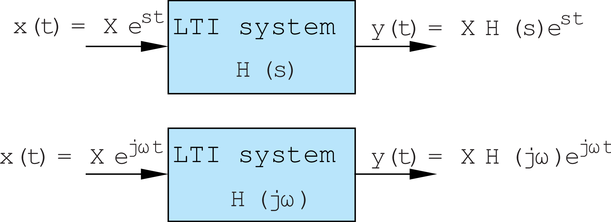
As we will see below, H(j \omega) is the "frequency response" of our system, meaning it tells us about the response to input sinusoids as a function of sinusoid frequency \omega = 2 \pi f, where f is frequency in Hertz. We can also characterize a feedback system's frequency response the same way,
While it is simple to substitute j \omega for s in formulas for H(s), the meaning of that substitution bears more study. In what follows, we try to do just that.
Examples
When we relate Y = H(s) U
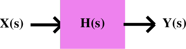
Examples:
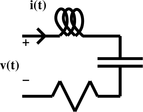
I(s) = Y(s) V(s) = \frac{1}{Ls +\frac{1}{Cs} + R} or V(s) = Z(s) I(s) = (Ls +\frac{1}{Cs} + R) I(s)
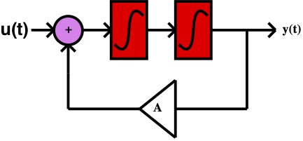
Y(s) = H(s) U(s) = \frac{1}{s^2 + A} U(s)
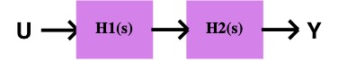
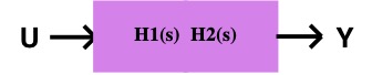
Composing Systems
W(s) = H_1(s) U(s) \;\;\;\; Y(s) = H_2(s) W(s) \;\;\;\; Y(s) = H_2(s) H_1(s) U(s)
Careful when modeling systems with bidirections coupling (like electrical circuits). A single block in our block diagrams is uni-directional (though if feedback is used, the entire diagram might not be uni-directional). That a block is unidirection means that the inputs to a block diagram are not directly effected by the block's ouput. So for example,
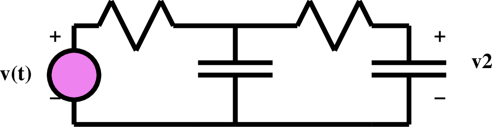
is NOT NOT NOT described by
V_2(s) = \left(\frac{1}{R_1 C_1 s + 1}\right) \left( \frac{1}{R_2 C_2 s + 1} \right) V(s)
because the left R-C circuit "loads" the right RC circuit.
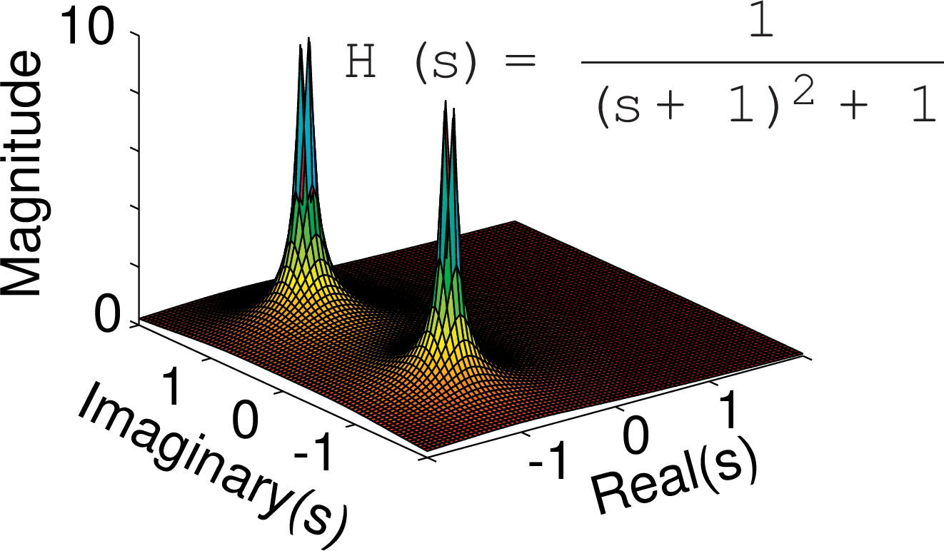
The system function H(s)
Real and complex poles
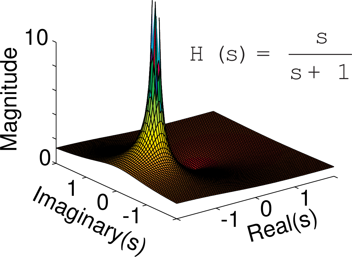
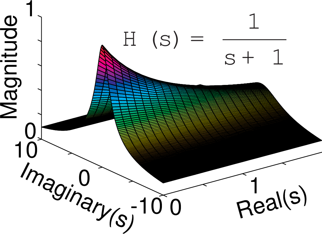
$H(s)$ is a complex function of a complex variable $s$. The plots show $|H(s)|$.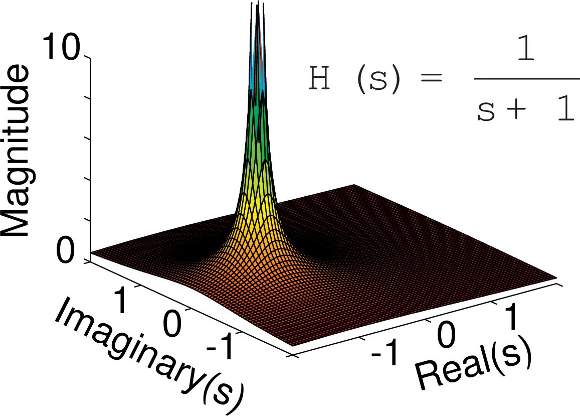
Effect of a zero
Interpretation of $H(s)$ by pole and zero vectors
In general, an $H(s)$ that is a rational function has the form $$ H(s) = K {(s - z_1)(s-z_2)\cdots(s-z_M) \over (s - p_1)(s-p_2)\cdots(s-p_N)} . $$ Thus, $H(s)$ consists of products and quotients of the form $$ (s- s_k). $$ Each of these terms are vectors in the complex $s$ plane.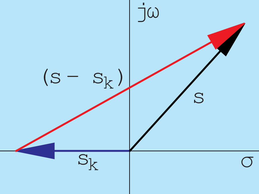
Therefore,
consists of products and quotients of vectors, i.e.,
so that
and
and
Frequency response
Relation to system function
Note that for
H(s) along the imaginary axis
We shall examine H(s) for s = j\omega or H(j\omega) where \omega is the radian frequency.
H(s) evaluated along the imaginary axis is called the frequency response.
Radian frequency and frequency
- \omega is the radian frequency in units of radians/second.
- \omega can be expressed as \omega = 2\pi f.
- f is the frequency in units of cycles per second which is called Hertz (Hz).
- The frequency response H(j2\pi f) is often plotted versus f.
Measurement of H(j\omega)
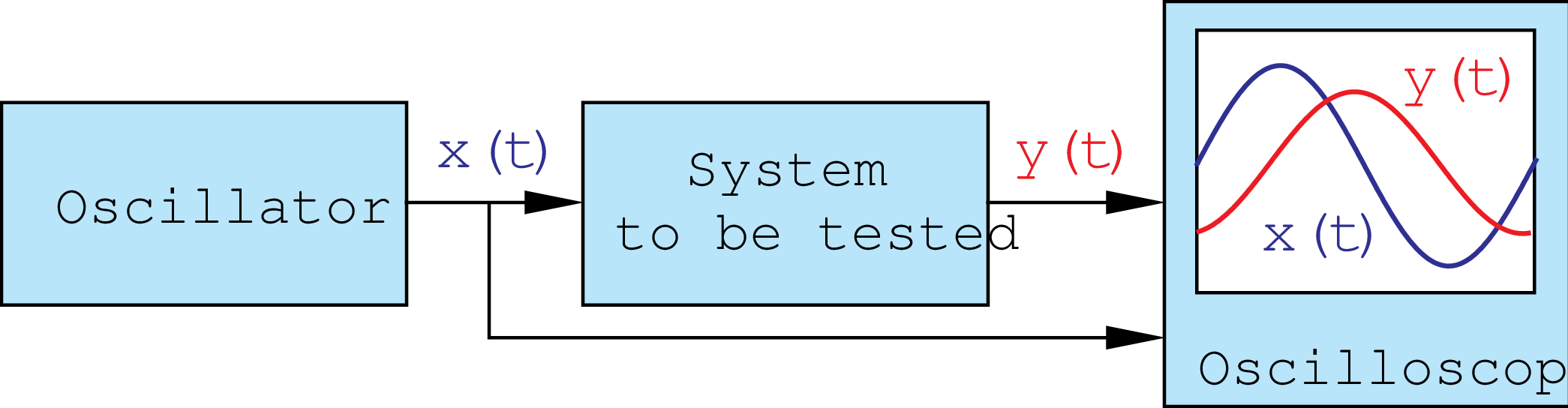
To measure H(j\omega) of a test system we can use the system shown below.
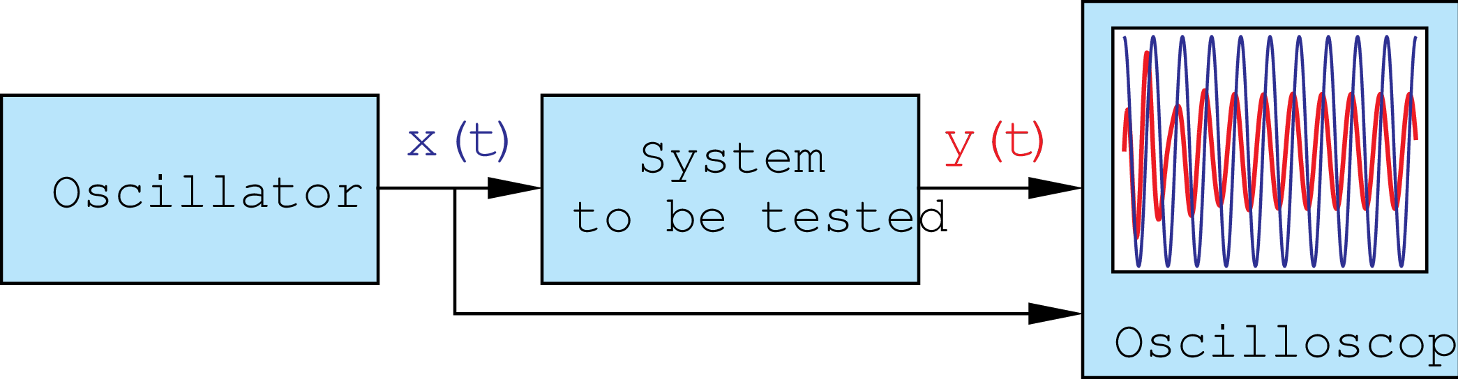
However, when the sinusoid is turned on the response contains both a transient and a steady-state component. For example, suppose
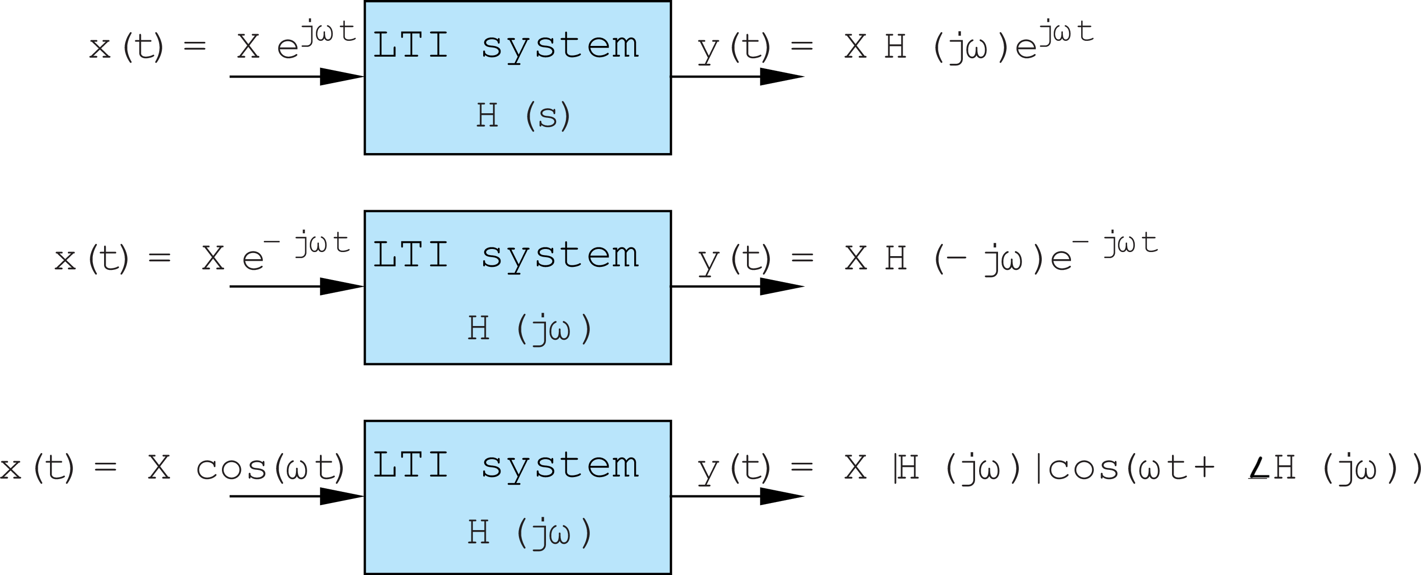
Therefore, to measure H(j\omega) we turn on the oscillator and wait till steady state is established and measure the input and output sinusoid. At each frequency, the ratio of the magnitude of the output to the magnitude of the input sinusoid defines the magnitude of the frequency response. The angle of the output minus that of the input defines the angle of the frequency response.
More elaborate systems are available for measuring the frequency response rapidly and automatically.
Relation of time waveforms, vector diagrams, and frequency response
Consider and LTI system with system functionThe input is
and the response is
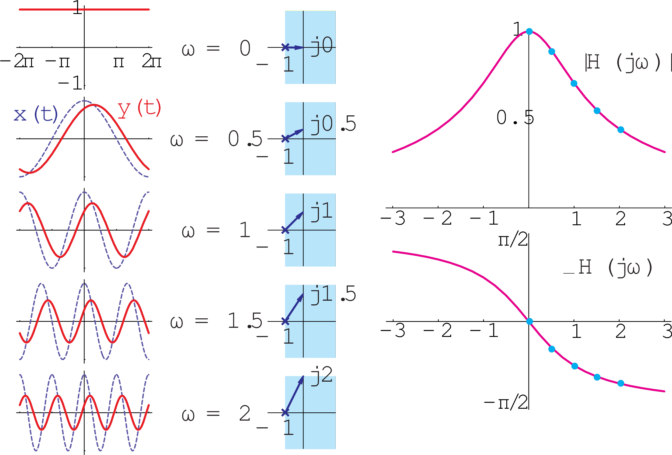
Different ways of plotting the frequency response
The frequency response $H(j\omega) = 1/(j\omega + 1)$, is plotted in linear coordinates on the left and in mostly log coordinates (the Bode diagram) on the right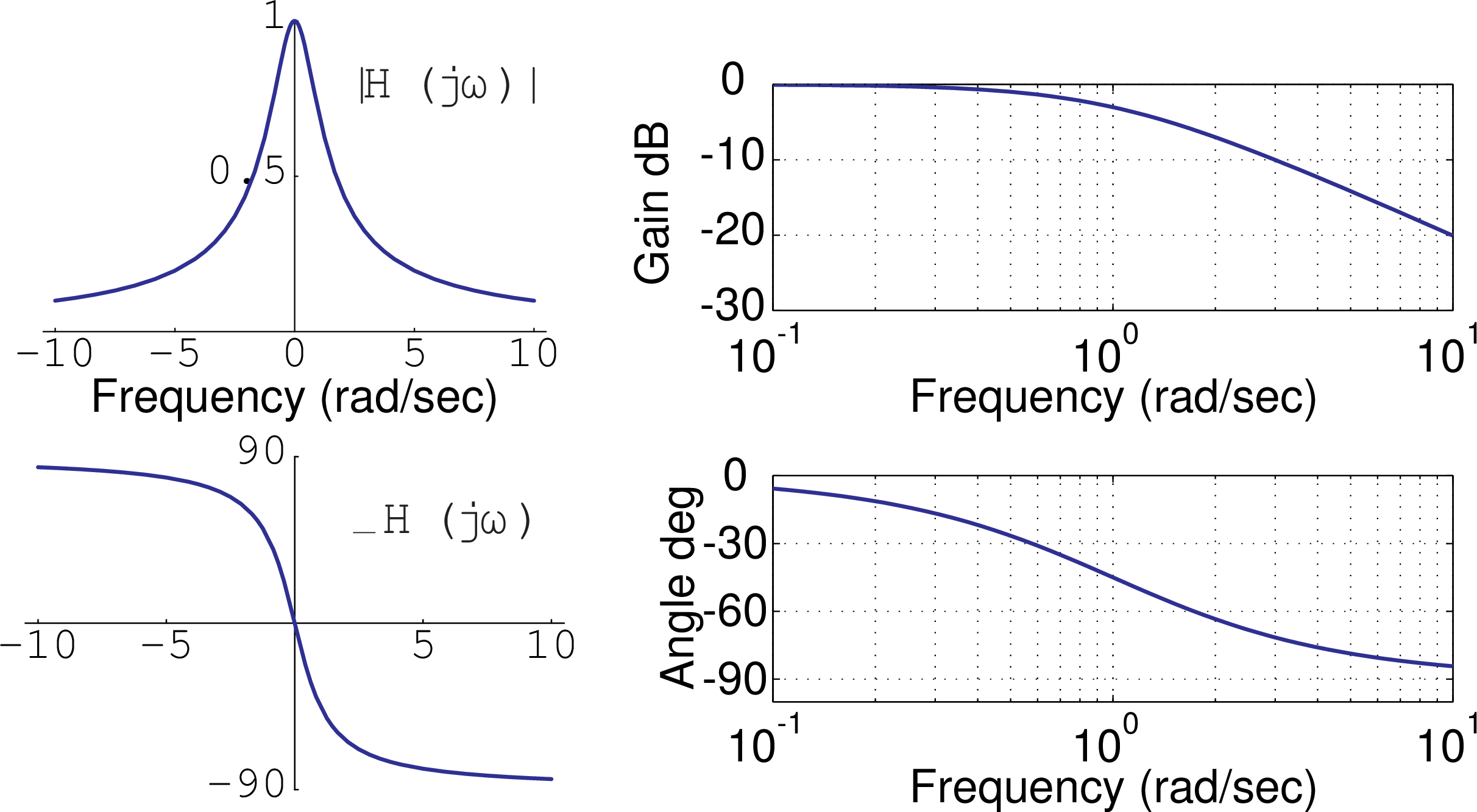
Bode diagrams
Definition and rationale
Frequency responses are commonly plotted as Bode diagrams which are plots of20 \log_{10} |H(j\omega)| is plotted versus \log_{10} \omega (log-log).
\angle H(j\omega) is plotted versus \log_{10} \omega (log x - linear y).
The reasons are:
- Logarithmic coordinates are useful when the range of |H(j\omega)| and/or \omega is large.
- Asymptotes to the frequency response are easily plotted.
- When the poles and zeros are on the real axis, the asymptotes are excellent approximations to the frequency response.
Pole-zero and time-constant form
Consider an LTI system whose system function has poles and zeros on the negative, real axis. It can be displayed in pole-zero form as follows
Magnitude and angle
The magnitude as a function of frequency $\omega$ can be expressed as a ratio of products,and the angle can be represented as the difference of sums
Logarithmic magnitude
Taking twenty times the logarithm of the magnitude yields
Note than both the logarithmic magnitude and the angle are expressed as sums of terms of the form
Decibels
It is common to plot frequency responses as Bode diagrams whose magnitude is expressed in decibels. The decibel, denoted by dB, is defined as $20 \log_{10} |H| $. Decibel equivalents for a few quantities.- |H| \rightarrow 20\log_{10}|H| dB
- 10^n \rightarrow 20n dB
- 2 \rightarrow \approx 6.02 \approx 6 dB
- 5 \rightarrow \approx (20 - 6) =14 dB
- \sqrt{2} \rightarrow \approx 6/2 = 3 dB
- 1.12 \rightarrow \approx 1 dB
How many decibels correspond to |H| = 50? Express |H| = 100/2. Then 20\log_{10}(100/2) = 20\log_{10}100 - 20\log_{10}2 \approx 40 -6 = 34 dB.
Corner frequency
At $\omega = \omega_c = 1/\tau$, called the corner or cut-off frequency,- the low- and high-frequency asymptotes intersect,
- the magnitude is
\pm 20\log_{10}|1 + j\omega \tau| = \pm 20\log_{10}|1 + j1| = \pm 20\log_{10} \sqrt{2} \approx \pm 3 \; dB,
- the angle is
\pm \angle (1 + j\omega \tau) = \pm \angle (1 + j) = \pm \pi/4 .
Example --- first-order lowpass system
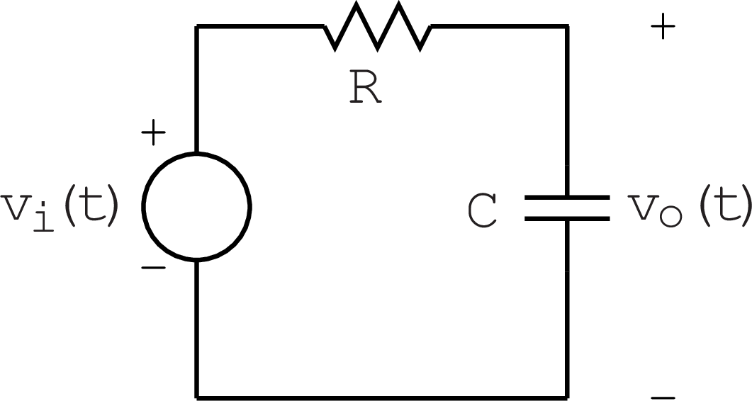
First-order lowpass systems arise in a large variety of physical contexts. For example,
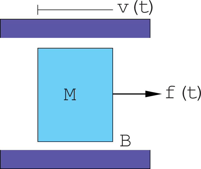
For the parameters M=B=R=C=1, the frequency responses for the two systems are
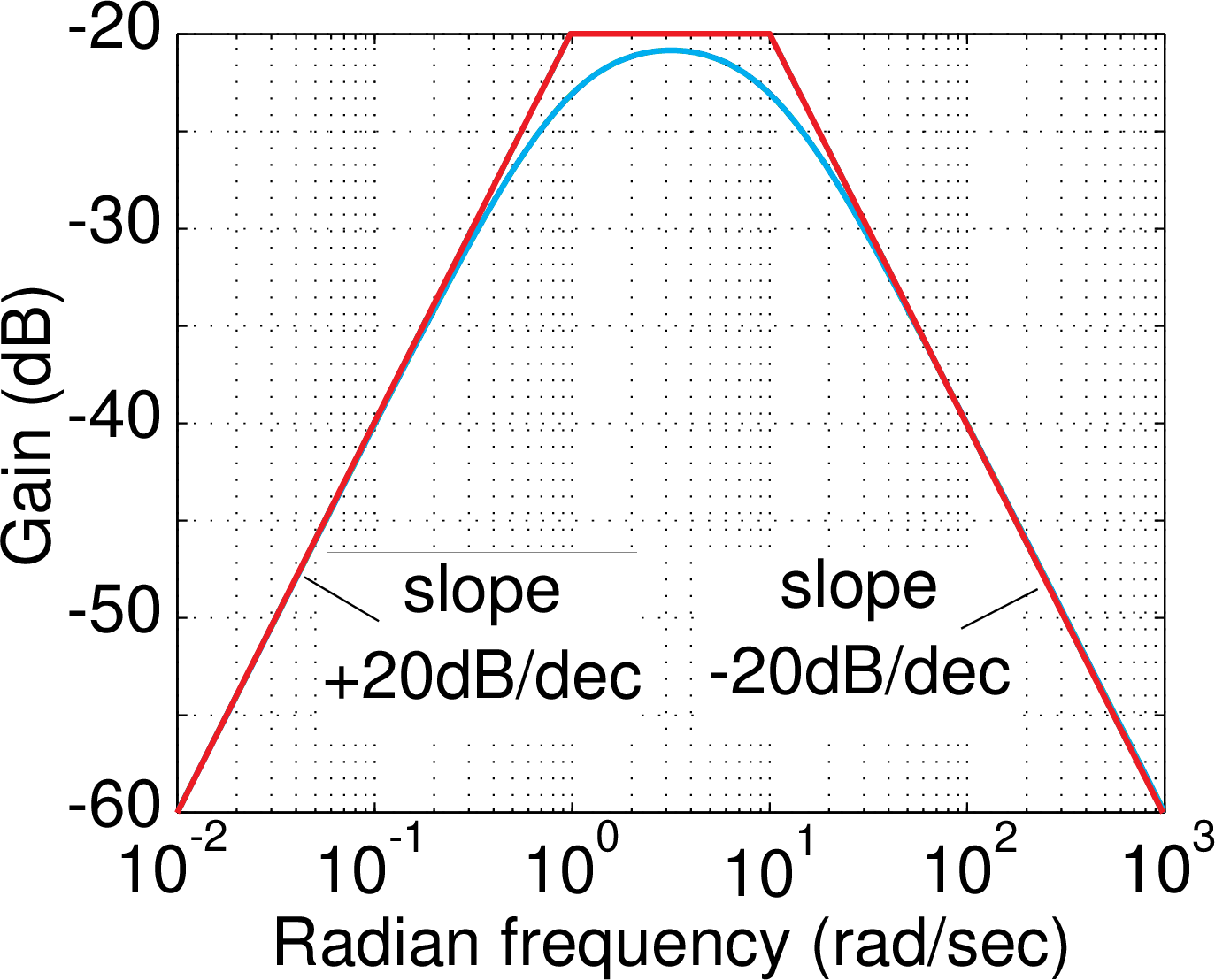
Magnitude
For $$ H(j\omega) = {1 \over j\omega +1} , $$ the low-frequency asymptote has a slope of 0 and an intercept of 0 dB and the high-frequency asymptote has a slope of -20 dB/decade and an intercept of 0 dB at the corner frequency.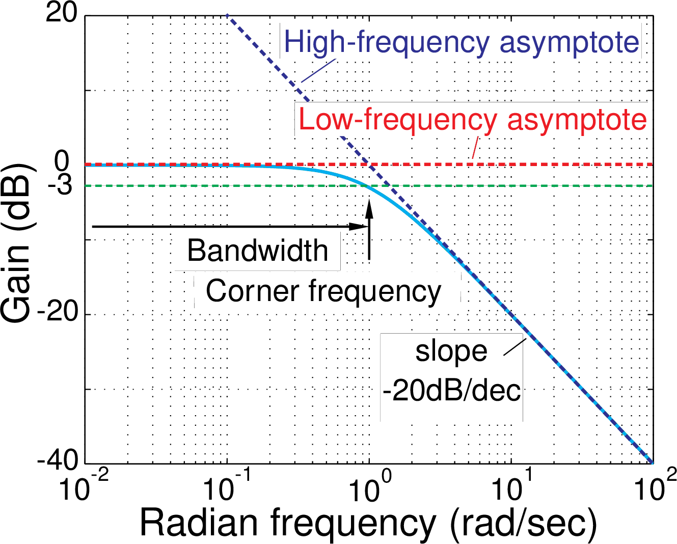
Angle
For $$ H(j\omega) = {1 \over j\omega +1} , $$ the low- and high-frequency asymptotes of the angle of the frequency response are 0 and $-90^{\circ}$ ($-\pi/2$ radians), respectively. The angle is $-45^{\circ}$ at the corner frequency (1 rad/sec).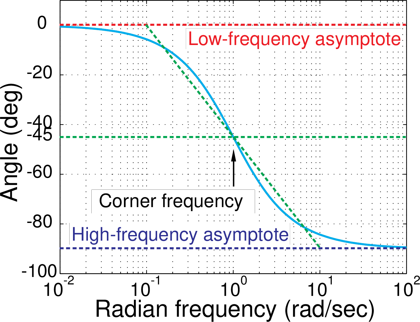
Physical interpretations
With M=B=1, the frequency response is
At high frequencies, |H(j\omega)| \rightarrow \frac{1}{\omega} and \angle H(j\omega) \rightarrow -90^{\circ}. The inertia of the mass dominates so that the acceleration is proportional to external force and the velocity decreases as frequency increases.
With R=C=1, the frequency response is
At low frequencies, |H(j\omega)| \rightarrow 1 and \angle H(j\omega) \rightarrow 0. The impedance of the capacitance is large so that all the input voltage appears at the output.
At high frequencies, |H(j\omega)| \rightarrow 1/\omega and \angle H(j\omega) \rightarrow -90^{\circ}. The impedance of the capacitance is small so that the current is determined by the resistance and the output voltage is determined by the impedance of the capacitance which decreases as frequency increases.
Miniproblem
Given
Summary
The frequency response
- is the system function evaluated along the j\omega-axis,
- has a simple geometric interpretation in the s-plane,
- describes the sinusoidal steady state response of an linear time-invariant system to an input sinusoid,
- has asymptotes that are easily sketched in a Bode diagram when the poles and zeros lie on the negative real axis.
Summary Questions
A linear, time-invariant, continuous-time system is described by its system function:
