Lab 5:
Win, Place, LQR
Please Log In for full access to the web site.
Note that this link will take you to an external site (https://shimmer.mit.edu) to authenticate, and then you will be redirected back to this page.
Quick Reference
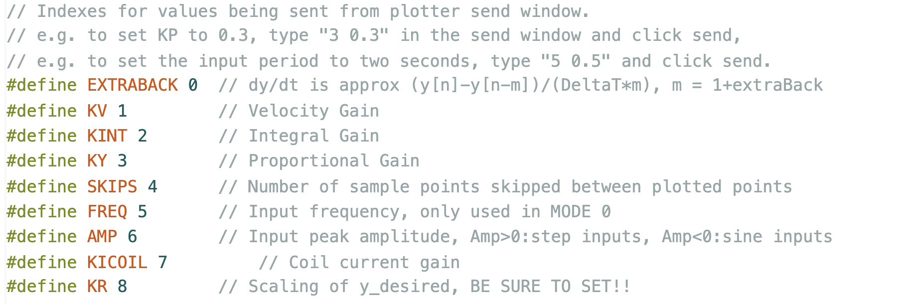
Serial Plotter Send Window Indices
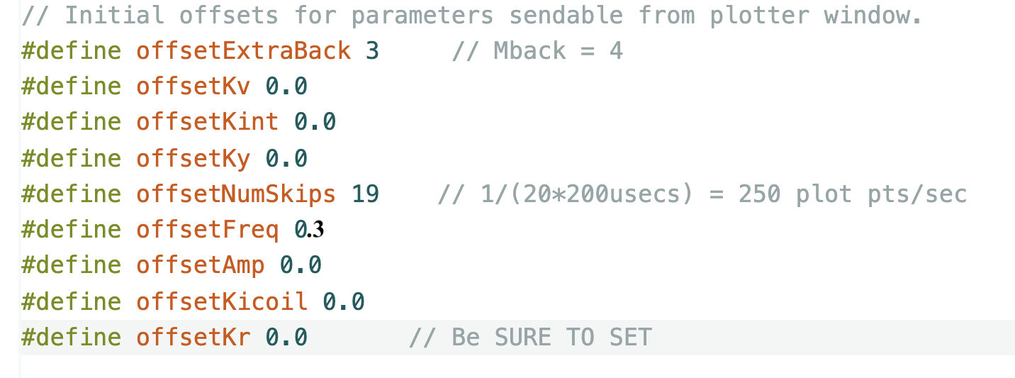
Useful Offsets to Set
Links
Task Summary
Week A:
- Add three magnetic pins to your umbrella.
- CALIBRATE your system's sensors (Checkoff 1).
- Download this lab's Teensy sketch (WHICH IS DIFFERENT FROM THE PREVIOUS MAGLEV Sketch).
- Ensure the fields of the three electromagnets are aligned.
- Calibrate
SensorOffsetandSensorScale. - Set the sign,
crntSign,and offset,crntOffset,for the coil current sensor.
- Determine and test a state-space model for the maglev system (Checkoff 2).
- Download the python script above, fix the TODO issues.
- Fill in A, B, and C matrices for your state-space model.
- Determine K and K_r for a PD-like controller in python and then copy over to the Teensy sketch.
- Verify that the python simulation matches measured maglev responses. Pay particular attention to matching both the dynamic AND steady-state behaviors.
- Try to design a state-space controller using pole placement (Checkoff 3).
- In the python script, set
useKyForKrto false anduseKplaceto true, then address the TODO issues in the python script for checkoffs one through three. - Use the script with pole placement to determine state feedback gains.
- Find poles for which the python-simulated step response is reasonable AND the motor commands (u) are within reasonable limits.
- Copy and past the gains generated by python into the Teensy sketch (after line 24), and demonstrate that the gains are effective.
- Verify that the model and the results from your maglev system are still a reasonable match for the best pole values you found.
- In the python script, set
Week B:
- Use LQR to design and test your maglev controller (Checkoff 4).
- Find the issues in the python script.
- Use the LQR algorithm to determine gains that optimize the python-simulated step responses.
- Examine the phase margin for your controller.
- Demonstrate your controller on your maglev system. What happens when you add more magnetic pins?
- Add an Integral term to your state-space controller (Checkoff 5).
- Assess the performance of your controller on your maglev system (e.g. add pins, try taking larger steps, try sine wave inputs, etc.).
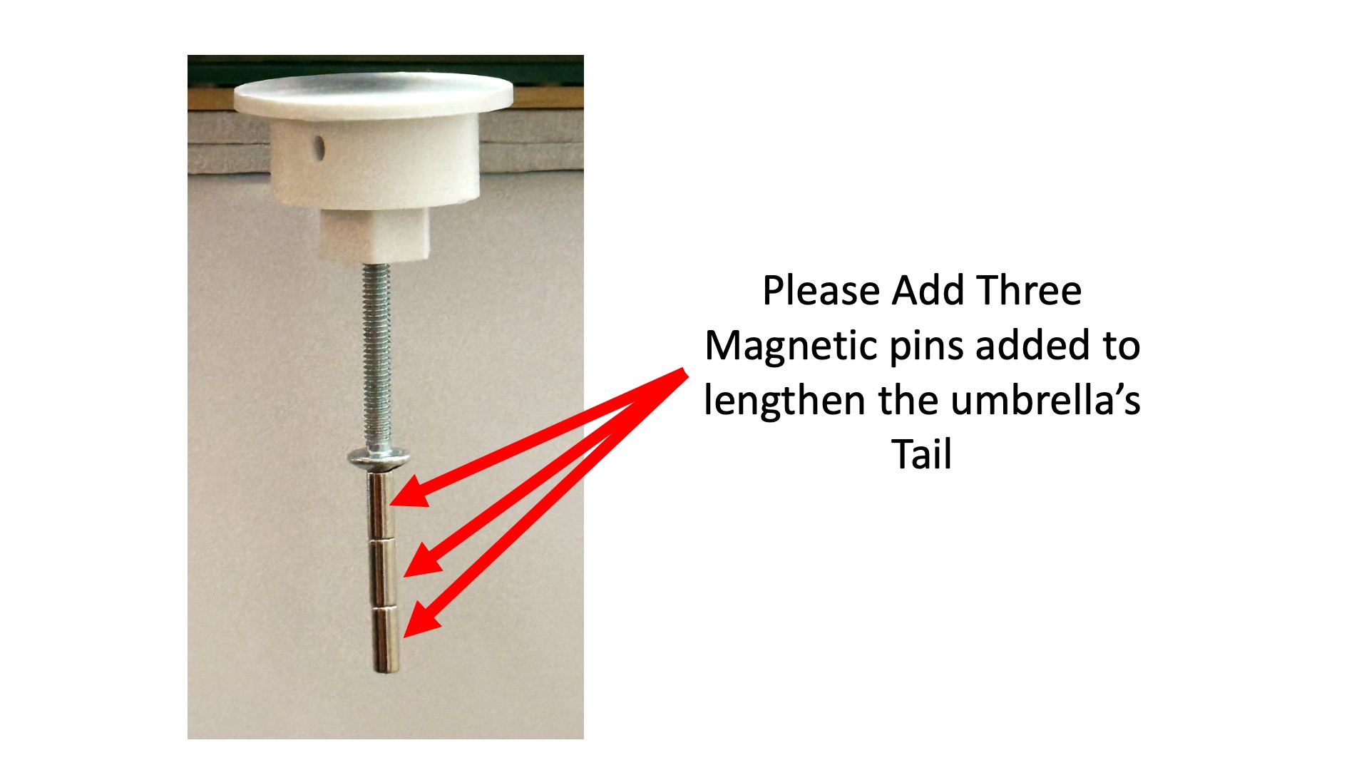
Add Magnetic Pins to Umbrella
Due to a change in the distance sensor positioning, the Fall 25 version of the maglev hardware is too sensitive to umbrella rocking. To reduce the rocking, please add a longer "tail" to the umbrella, by adding three pin magnets as in the picture below.
Sensor Calibration
Download this week's sketch and update the system parameters in this sketch to match your system as follows.
- Set the optical sensor parameters (
SensorScaleandSensorOffset). You can transfer the values from last week's sketch, but you should check the result by verifying thatDY_mis-1500or0when the umbrella is in the top or middle reference positions, respectively. - Check the polarity of all three coils using a compass. Correct the differences by swapping in the parameters in the
hbridgeBipolarstatement near line 205 in the Teensy sketch. - Check the polarity of the coil currents by viewing
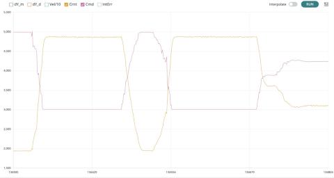
CrntandCmdwhile disabling the other traces. Turn the offset potentiometer back-and-forth from fully clockwise to fully counterclockwise. IfCrntsteps up whenCmdsteps up (left panel below), thencrntSignis correct. If the steps are in opposite directions (right panel below), change the sign ofcrntSignin line 13 of the sketch.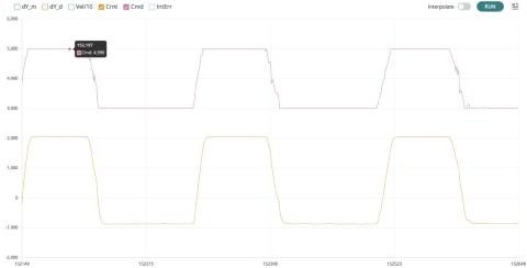
- Determine an offset for the coil current measurement so that the variable
crntwill be zero when suspendeding the umbrellad 1.5 centimeters below the bottom of the black maglev sensor-and-rod bracket. To find the offset,- Set both
Ky(index 3 in the send window) andKr(index 8 in the send window) to 2. - Find a value of
Kv(index 1 in the send window, and should be near 0.025, that's 0.025 NOT 0.25), and a setting for your offset potentiometer, so that your umbrella floats stably at distance zero as measured by the optical distance sensor. - DEBUG TIP: If your umbrella falls or slams into the black bracket, you may need to flip the sign of the feedback. To flip the sign of the feedback, you can either flip the umbrella magnet (ask for help) or change the directions of all the coils, i.e. switch B1L with B2L, A1L with A2L, and A1R with A2R, near line 205 of the Teensy sketch.
- IF YOU FLIPPED THE SIGN OF THE FEEDBACK BY FLIPPING THE DIRECTIONS OF ALL THREE COILS, YOU MUST RECHECK THE POLARITY OF CURRENT MEASUREMENT AS IN STEP 3 ABOVE!!!!!!!!!
- Set the current offset (
crntOffset) on line 15 of the sketch so that when the umbrella is stably suspended at distance zero, the coil current (Crnt) displayed on the plotting window is near zero (typical current offset values are between 0.2 and 0.8).
dY_d,dY_m, andCrntwhile the umbrella is hovering atdY_dnear 0. - Set both

Transferring to States
In this lab, you will be designing state-space controllers for your Maglev system, but you will not be starting over, as we hope to make clear in this section.
The Ins and Outs
In order to design a better-than-PD controller for our maglev system, we needed an accurate model. We used a combination of analysis and measurement to determine a transfer function model for the system, or more specifically, for the green encapsulated region in the maglev system diagram below.
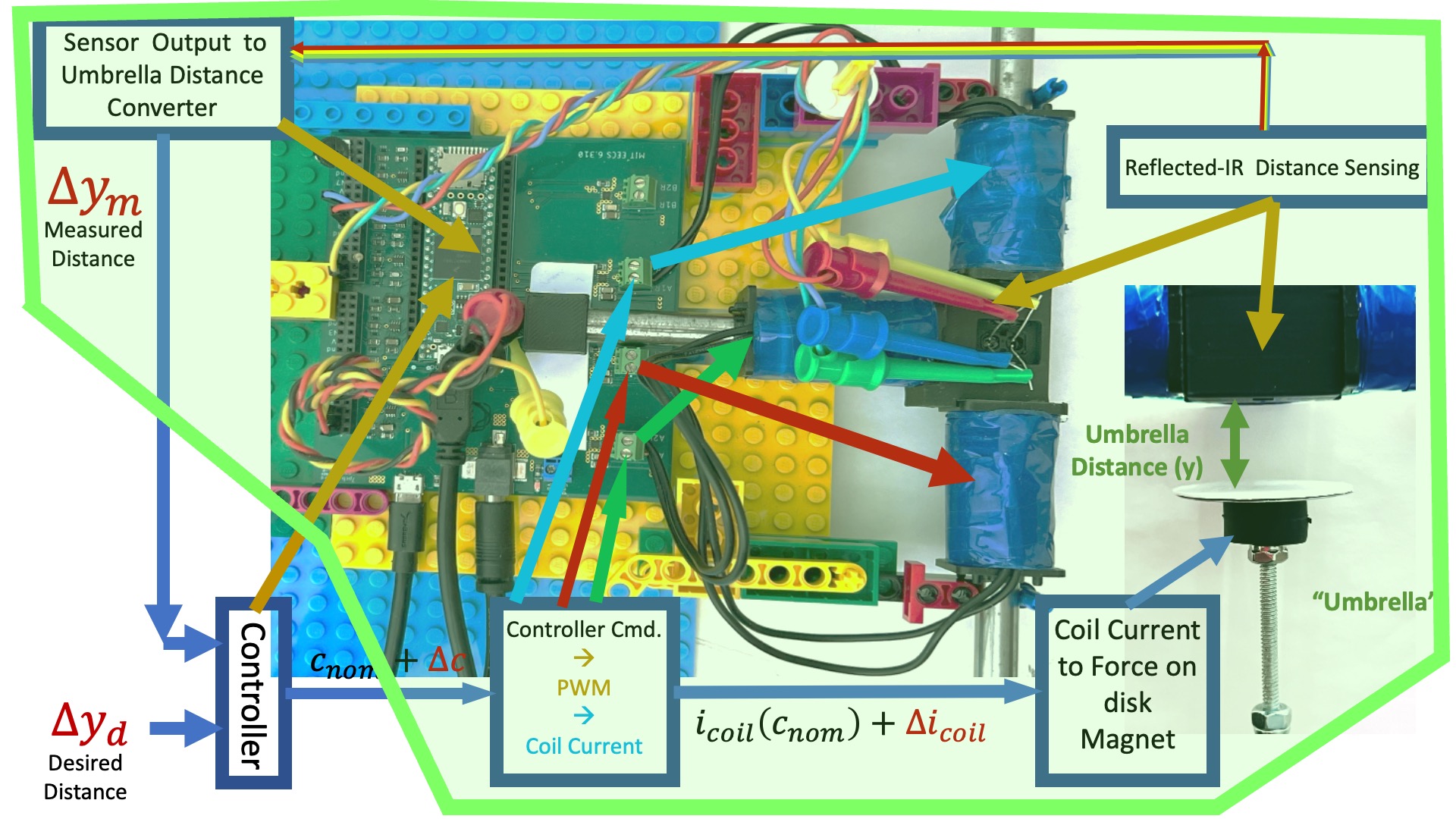
The single-input single-output maglev transfer-function model is shown in the block diagram below (and labeled H_{c2y}(s)), where it is combined with a "lead" controller, labeled K(s), and embedded in an umbrella-position-controlling feedback system.
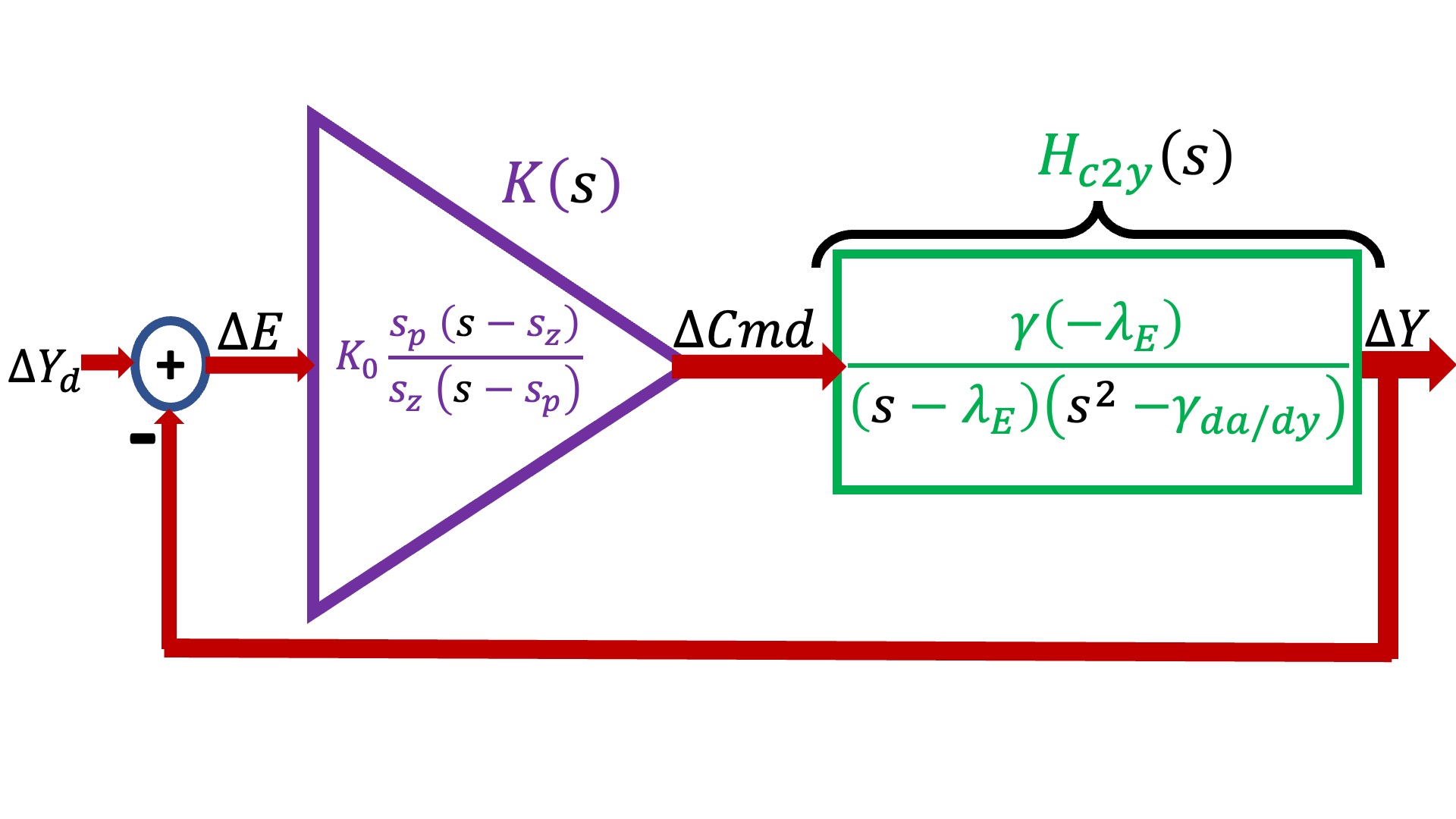
In the above block diagram, the maglev model (in green and labeled H_{c2y}(s)) has three model parameters, \gamma, \lambda_E, and \gamma_{\frac{da}{dy}}, and the lead controller (in purple and labeled K(s)), has three design parameters, s_z, s_p, and K_0. In the last lab, we used a variety of measurements to determine H_{c2y}(s)'s model parameters, and then used that calibrated model (along with the concept of phase margin) to determine K(s)'s design parameters.
State-ing the Obvious
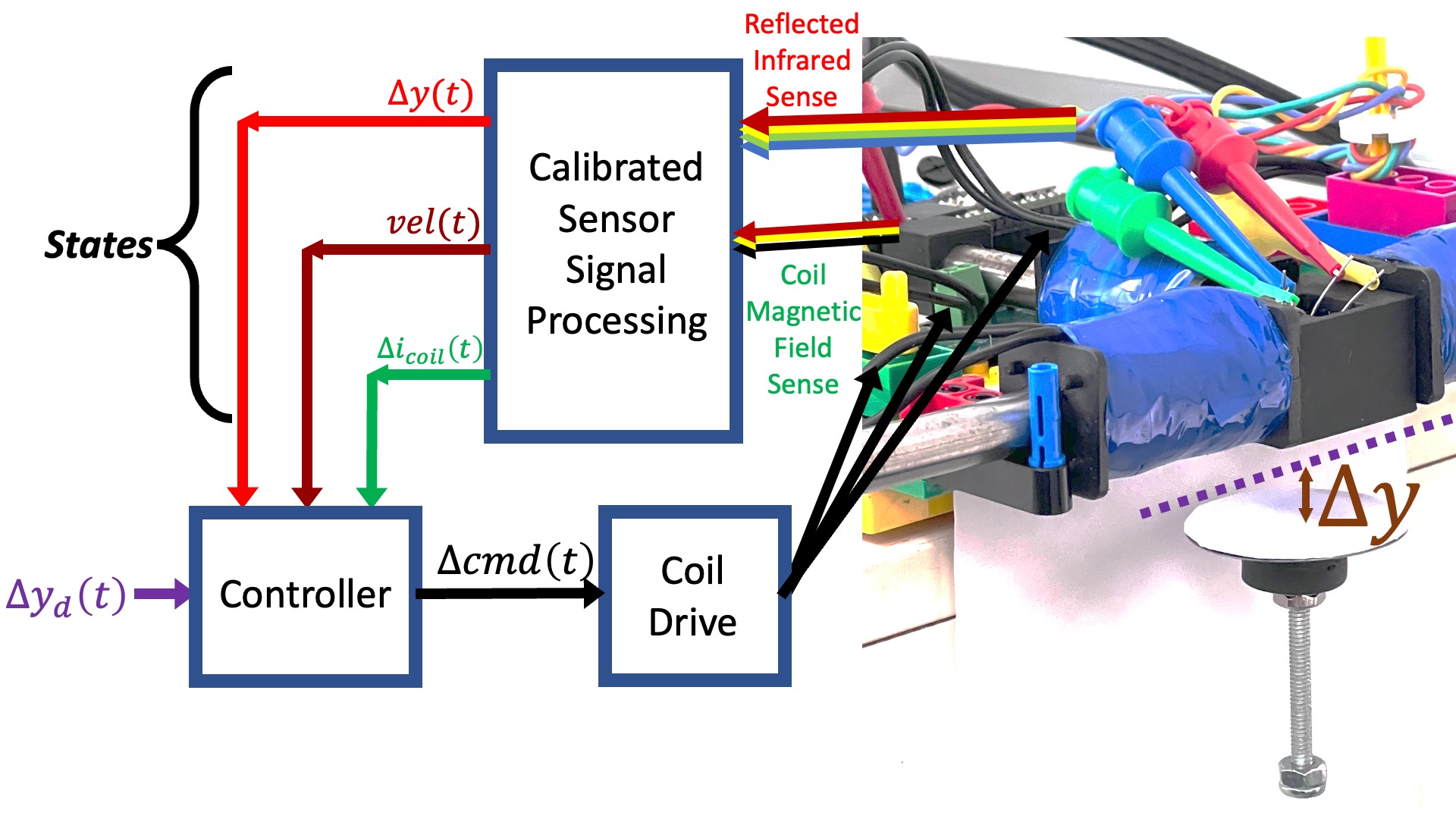
We are using an optical sensor to estimate umbrella position, are using its sample-to-sample variation to estimate time derivatives, and are using a magnetic field sensor to estimate coil currents. Effectively, we are measuring the umbrella's state: its position, its velocity, and its acceleration (coil current is proportional to force, force is proportional to acceleration). Yet we are not using state-space control, we are not even using all the states we can measure. Coil current is ignored by our PD and lead controllers, its measurements are only being used for model calibration.
As an alternative, consider the system diagrammed below, in which the controller uses measurements of coil current, umbrella velocity and umbrella position to determine command updates to the coil driver.
We could then use a linear state-space controller, like in the figure below.
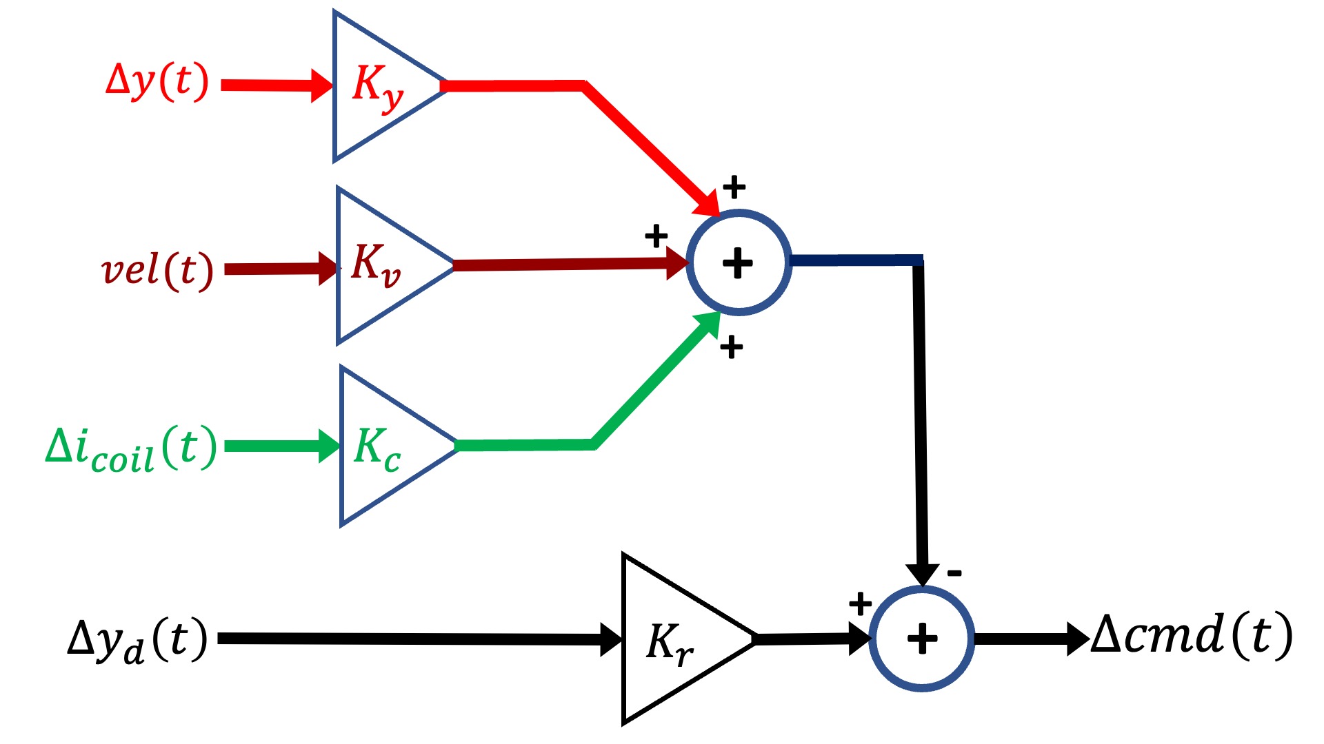
It was difficult enough to design the lead controller when we only had three parameters to determine, s_z, s_p, and K_0. And as the above diagram makes clear, we now have four, the three state "gains", K_y, K_v, K_c, and the input scaling, K_r. Luckily for us, there are computational tools that will help us find reasonable values for the K's, given a state-space model for our system.
State-Space
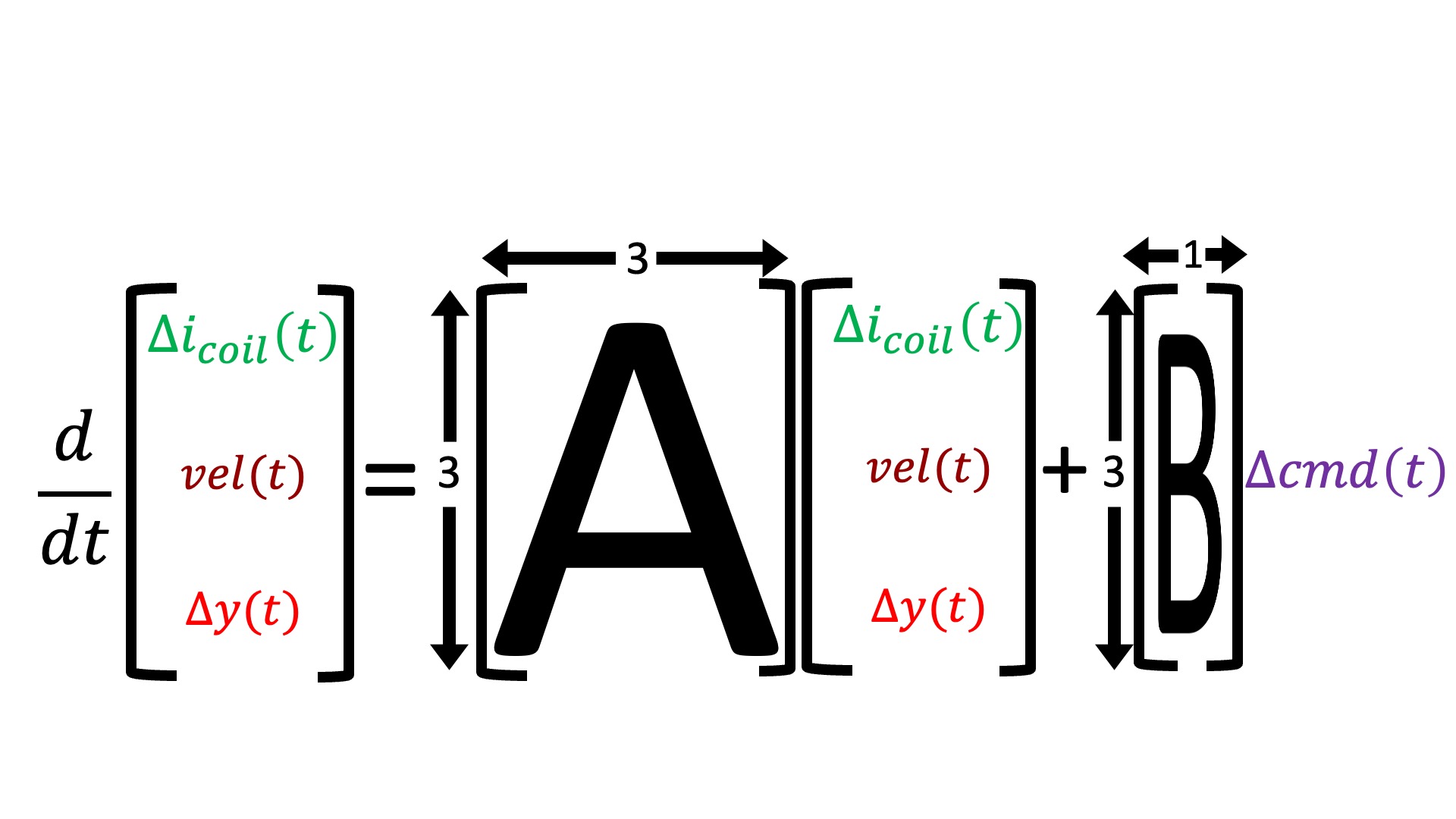
Consider the state-space model differential equation,
We summarize system with the states and matrices below.
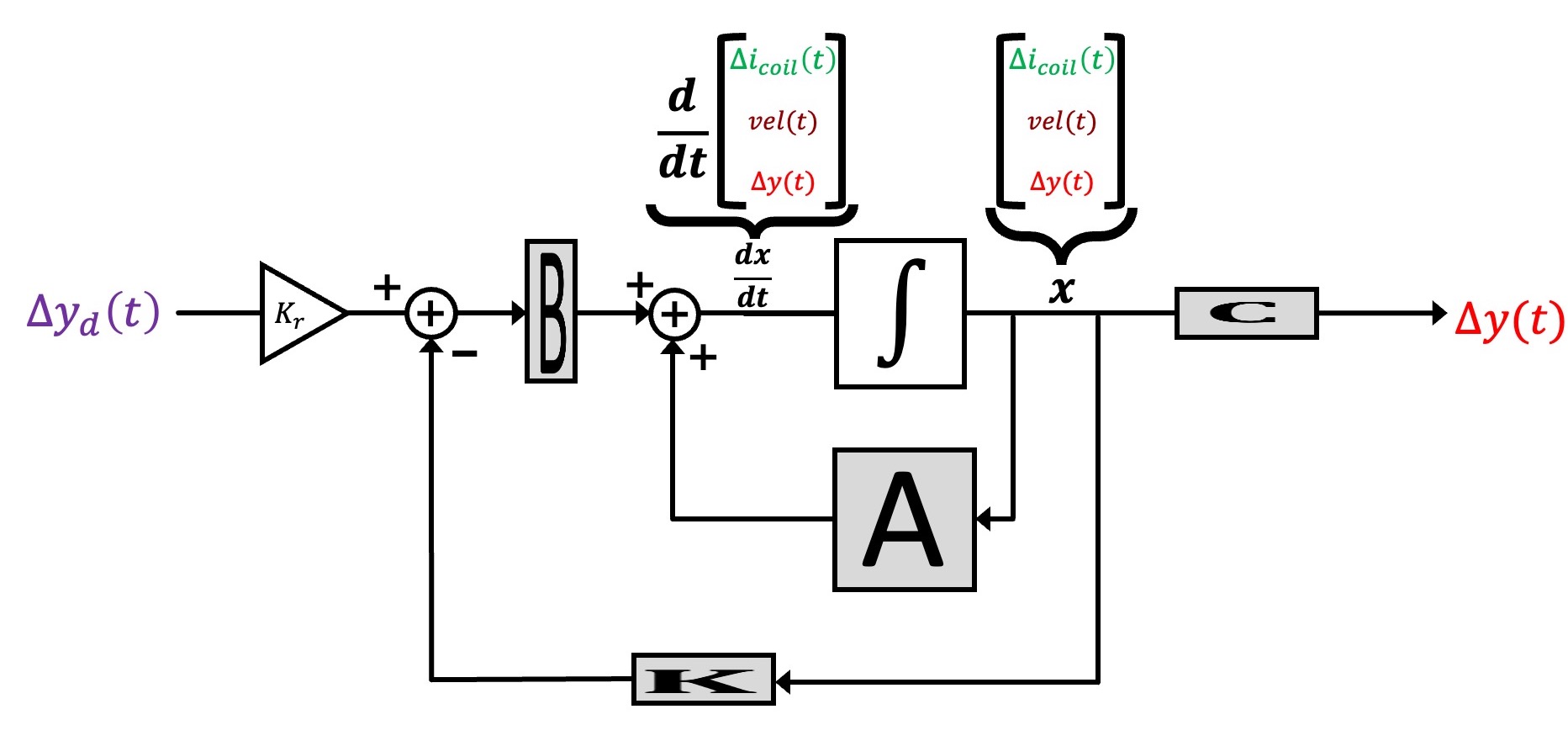
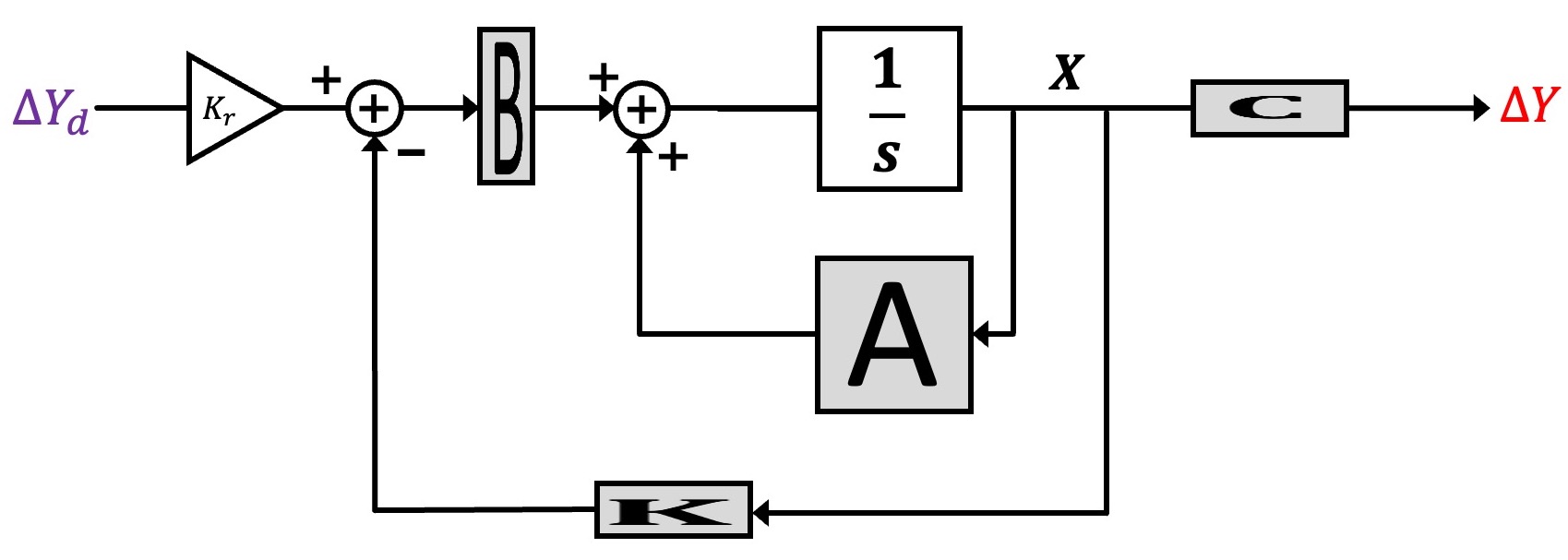
In standard state-space feedback, u(t) = \Delta cmd(t) is given by a scaling of a desired input, K_r \Delta y_d(t), minus feedback from a weighted combination of the states, -K x(t), as shown in the block diagram below.
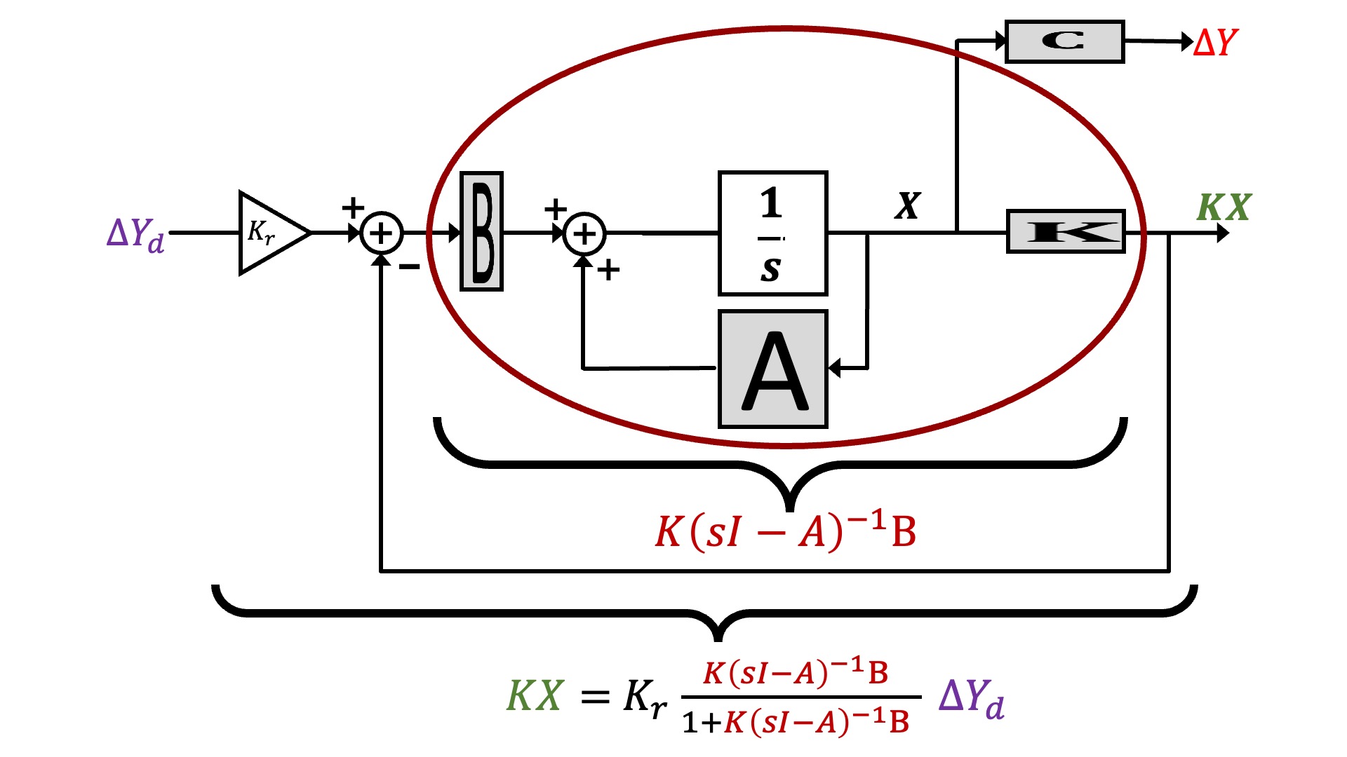
We can represent the block diagram in transfer function form, as shown below.
And finally, we can reorganize the state-space description to make its description look more like the feedback loops we have been analyzing with Black's formula, as shown below.
Consistent States
Fortunately, in the last lab we created and carefully-calibrated a model of our maglev system, but unfortunately, the model is in transfer-function rather than state-space form. And transforming the transfer-function model to a state-space model requires that we pick states consistent with our measurements. Tackling this problem will be this lab's first challenge.
Determining and testing the state-space model.
What we need is a state-space model whose states are consistent with our measurement of umbrella position, umbrella velocity, and coil current. That is, we must find an \{A,B,C,D\} state-space model for our maglev system that satisfies two criteria:
- its states are umbrella position, umbrella velocity, and coil current;
- its transfer function matches your carefully-calibrated maglev transfer function from the last lab.
The First Row
To start the process of mapping the transfer function into the A and B matrices in the above figure, consider unraveling the H_{c2y}(s) transfer function back into a product of two transfer functions, one from Teensy command to coil current and one from coil current to umbrella position as shown below.
As noted in the above figure, we now have an explicit \Delta I_{coil} and an explicit \Delta Y that correspond to the first and third states, but we do not have anything explicit relating to velocity. Nevertheless, from H_{c2i}(s) we can determine the differential equation that relates Teensy command to coil current, and map its coefficients into the appropriate matrix elements in the first row of A andB, as shown in the figure below.
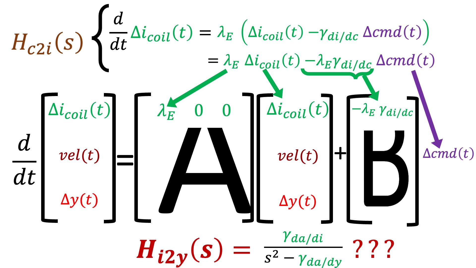
In the above two figures, we noted that velocity is missing in the transfer function and H_{i2y}(s) is unused in constructing the state-space model. How might we incorporate this unsed information to fill in the bottom two-thirds of A and B?
BONUS TIP: There are a few tricks to converting transfer functions to state-space models,reviewed in the prelab question here.
The Python Script
We have provided a Python script with the structure of a state-space model for maglev. To use the script to model your hardware system, you will have to provide values for several parameters, including \lambda_E, \gamma, \gamma_{da/dy} and scale. Note how scale is used to compute \gamma_{da/di} and \gamma_{di/dc}, do you see how to use scale to change the scaling of i_{coil}. You will need to use that insight below.
You have already measured several of these parameters in last week's lab, but since we changed the umbrella slightly (adding pins), your model will need updating. Take some time to examine the script and make sure you understand what each part is doing.
Note that we created a system with multiple outputs, defined by the matrix Cplot in the python script. We did this so that when we used the step (Python), plots of all three states are generated, not just position. But we also want to plot one more quantity. Recall that u = K_r y_d - K x, and that in our case, u = \Delta cmd, and its plot should not exceed 10 by much, or be much smaller than -10 (\Delta cmd will saturate the coil driver if outside the range -1 to 1, and we scale that by 10 because the script is simulating a unit step, and we typically take steps of 0.1). The step function will plot u = K_r y_d-K x if we prepending a row to the Cplot matrix and add a single non-zero value to a 4 \times 1 Dplot matrix.
For state-space models, D is used to represent a direct contribution of system's input to its output, as in
Modeling and Matching (Checkoff 2)
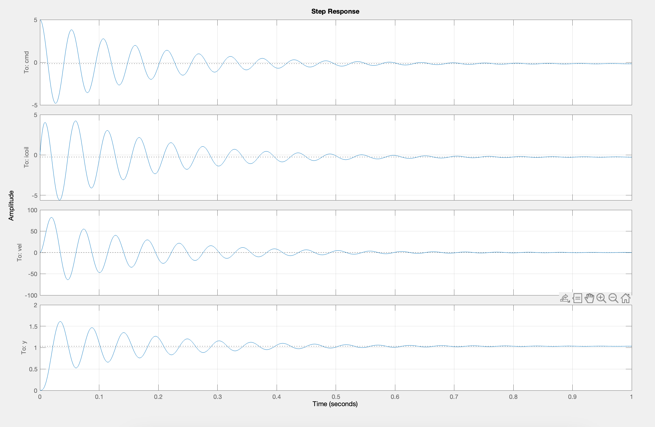
Please use your insight into state-space modeling, along with the hints above, to find and fix the lines associated with TO DO in the Python script linked at the top of this page. For a quick summary of the formulas for computing closed-loop matrices, look here. If you have a reasonable state-space model and you set values for K and K_r that are consistent with the PD controller you used above (though we suggest you use a small enough value of K_v so that your maglev system's step responses have oscillations, then after running the script you should see four plots. From top to bottom they are: the Teensy command being sent to the maglev coil drivers, i_{coil}, vel and y.
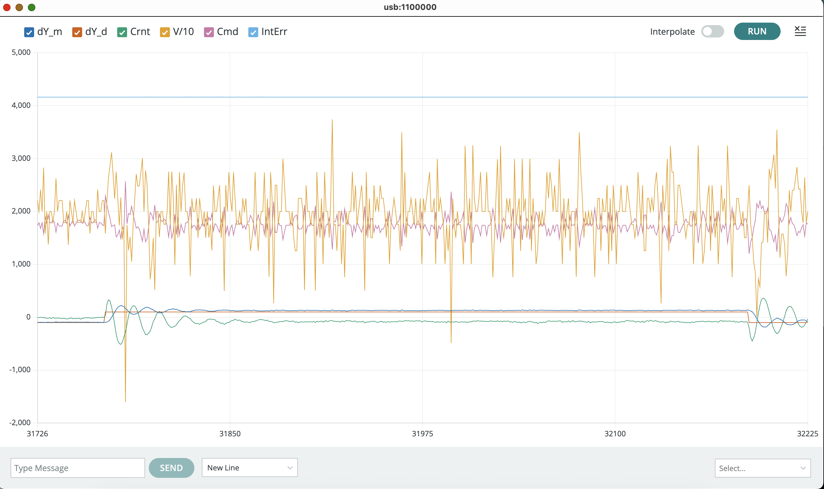
Once you have the python script producing reasonable outputs, copy and paste the python-produced #define statements lines from the python command window into the Teensy sketch (after line 24). Plug in both board power supplies, connect your laptop to the Teensy, and upload the Teensy sketch, and start the serial plotter. When you start the serial plotter, you should see a plot of six waveforms (this time starting from the bottom and working up): \Delta y, the umbrella position; \Delta y_d, the desired position; vel, the umbrella velocity; Crnt, the electromagnetic coil current; Cmd, the Teensy command to the coil driver; and intErr, the integral of the position error. A typical plot snapshot is shown in the figure below. Notice that the controller update period is 200\,\mus and numSkips starts out as 19. Therefore, there are 250 plotted points per second by default.
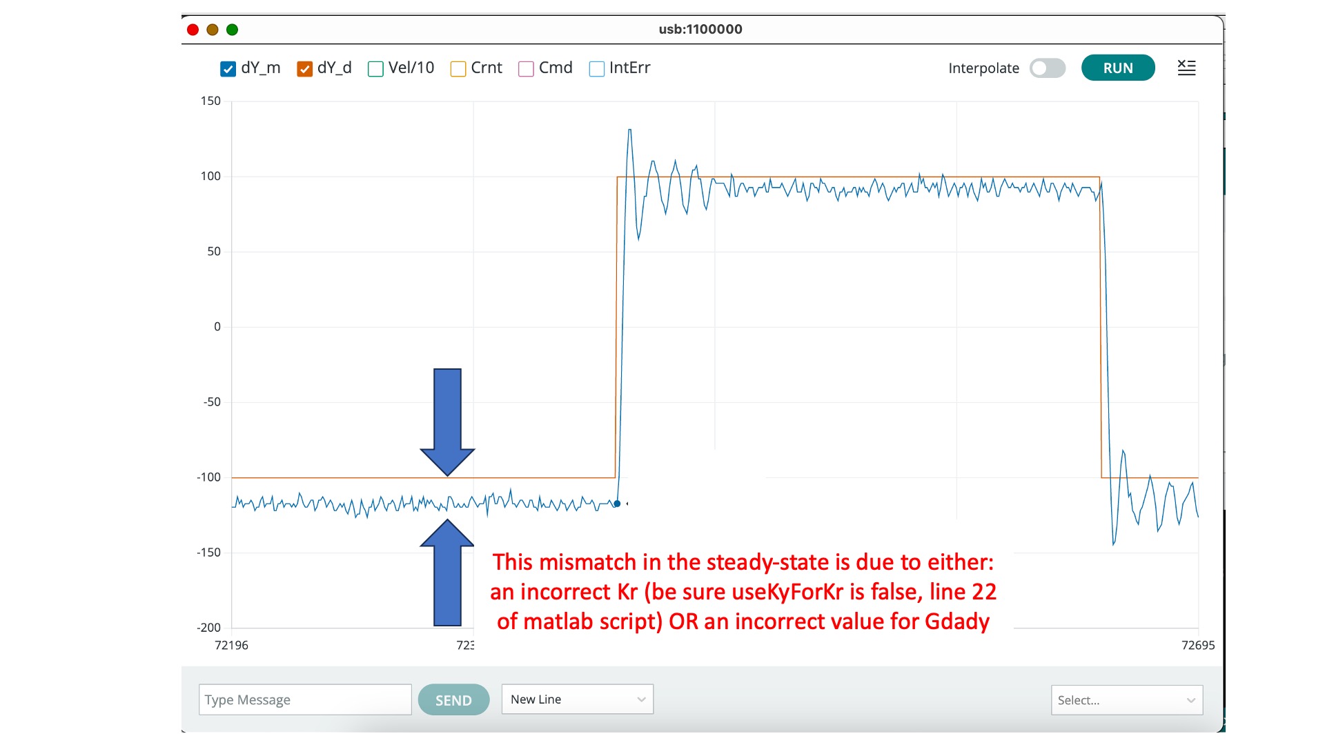
In the Teensy serial plotter, you can unclick all but \Delta y and \Delta y_d, to focus in on position errors, as shown below.
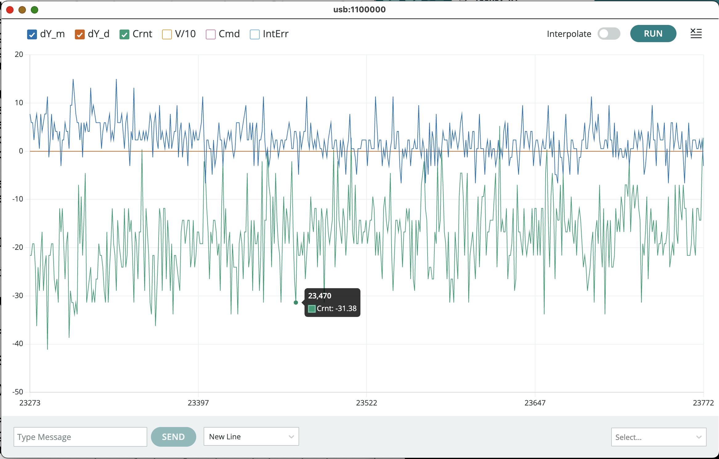
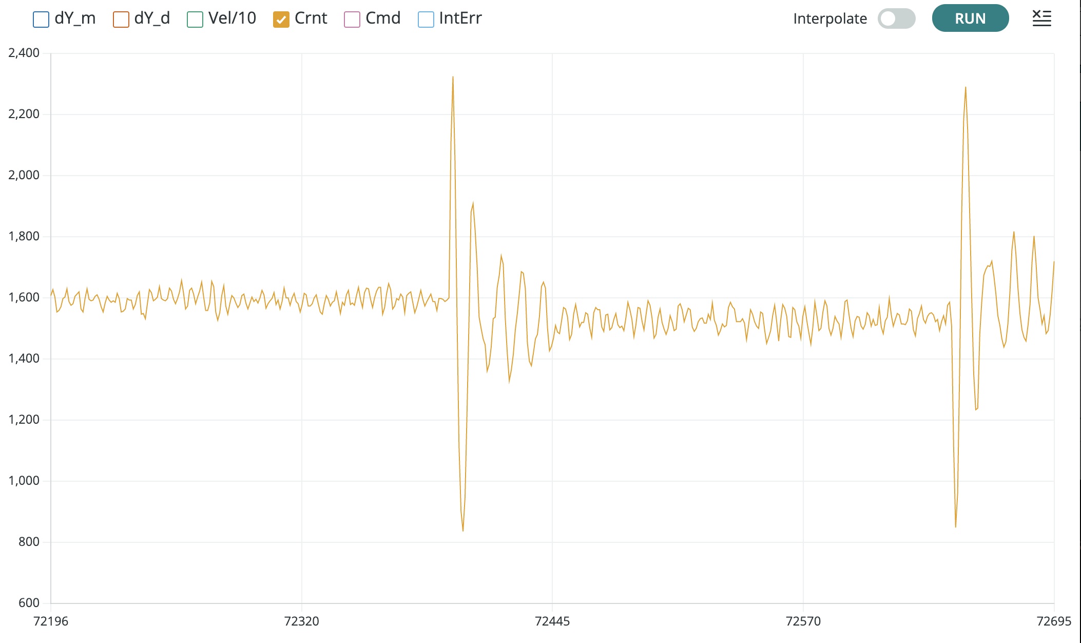
Or unclick all but Crnt to focus in on the coil current scaling, as shown below.
Now if you set the same K and K_r on your lab system, you should be able to compare the plots from the Teensy serial plotter to the simulation outputs from the script. If your model is a good match, then you should see results like the ones shown in the figures below. If the model and simulation are mismatched, tweak the model parameters until you get a good match. The better your model, the better the resulting controller.
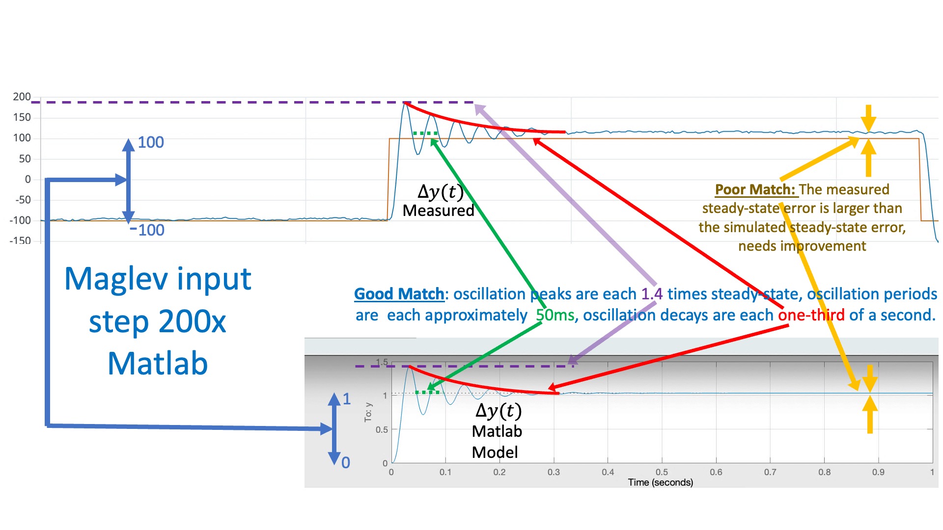
In the figure above, we compare the simulated and measured umbrella position, to check that they have the same "shape" (initial overshoot, oscillation period, oscillation decay time). Note that there is a scale factor between the plots that reflects a scale factor in step size. The script is using a "unit step", but when we set the square wave amplitude to 0.1 in the Teensy sketch, we can see (from the red y_d plot) that we generate a step of 200 (-100 to +100) in the units of the serial plotter. So the measured step is 200 times larger than the simulation (again in the plotting units).
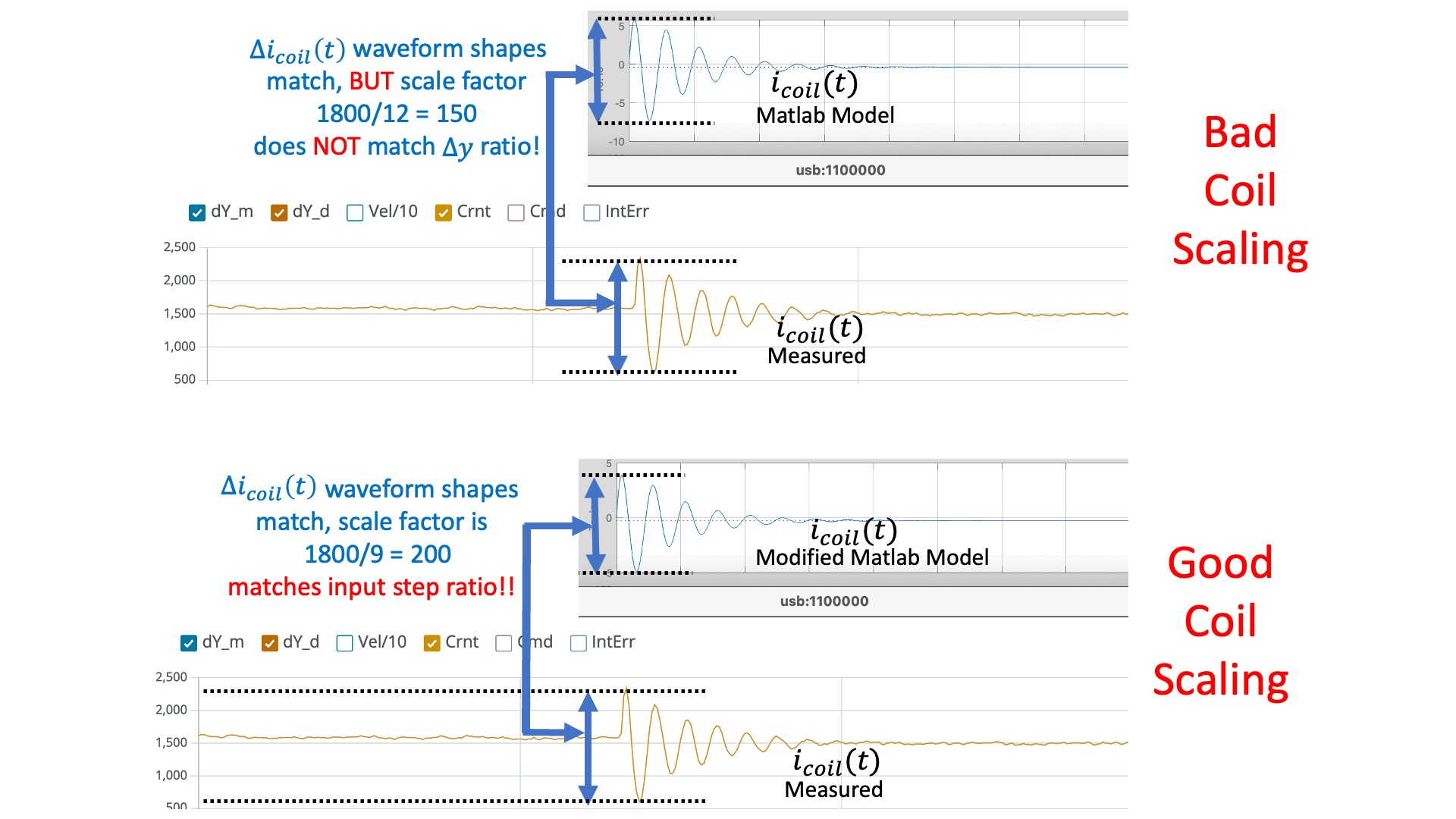
When comparing coil currents, as in the figure below, there should be the same scale factor of 200. So the measured current should have the same shape as the simulation, and should be 200 times larger.
Mismatched scale factors between measurement and model are BAAADDDD! If the scaling is not consistent in the model, then when you use that model to compute state feedback gains, those gains will be incorrectly scaled. And with incorrectly scaled gains, chances are your feedback system will be UNSTABLE!
DEBUG TIPS: Use low gains when trying to match model to measurements (e.g. Ky=2.0). Higher feedback gains will hide model details from you (that is the point of feedback). If your coil scale factor is off, you may need to slightly adjust scale in the python model. If your ringing frequency in simulation doesn't match your measured frequency, you may need to slightly adjust \gamma. If the decay rate of the oscillations does not match, you may need to adjust \lambda_E and if the steady-states do not match, you may need to adjust \gamma_{da/dy}.
Pole Placement
By providing feedback on all of the states of a plant, state-space controllers can offer significant performance improvements over what can be achieved with PID controllers. However, to realize these potential improvements, we must choose a gain for each state variable in the state vector x.
As you saw in the prelab, we can easily solve simple second order systems "on paper" and find gains that place the eigenvalues wherever we like (subject to a few constraints such as avoiding repeated eigenvalues). For larger systems, beyond third order, there is no closed form for the eigenvalues, and finding the gains for a given placement is best done computationally. We can rely on numerical approaches for determining K given \textbf{A} and \textbf{B}, such as Ackerman's method and its variants. Python's place command does exactly what we want, provided we do not try to place multiple poles with the same numerical value.
In the Python script, set be sure to set useKyForKr to false and useKplace to true!
Unfortunately, even though we have a function that will take desired eigenvalues (aka poles) and return the needed gains, that does not mean we can just set the closed-loop eigenvalues to be real and put them at -\infty. If we could, then our system would respond infinitely quickly to changes in desired position, and who wouldn't want that?
What happens when we make the poles too negative? What physical limitations stop us from choosing arbitrarily negative poles?
Use the pole-placement algorithm to find gains (K) as described in the following checkoff and then implement your "best" result with your maglev hardware. You can use the python script to run the pole-placement algorithm by setting the useKplace flag to true (near the top of the python script), and fixing all the appropriate to-dos.
Notice that the python script prints the gains in a format that can be copy-and-pasted directly into the Teensy sketch (after line 24 in the Teensy sketch). So, when transferring the K's you computed with the python script to the Teensy sketch, we STRONGLY recommend copy-pasting the gains from the script into the sketch and reuploading. PLEASE DO NOT TRY setting the four gains using four different indexes from the send window in the serial plotter. We do not display those values, so a mistake can easily go unnoticed.
Setting Gains with Pole Placement
END OF ASSIGNMENT FOR WEEK A
Using LQR
The pole-placement algorithm allows us to choose gains K to set the closed-loop poles anywhere we please. However, if the resulting performance has problems (e.g., if the umbrella settles too slowly or if the required commands are too large), it is not always obvious how to change the poles to improve performance. This issue can be addressed by using the LQR algorithm, which specifies gains using a different set of parameters.
We strongly recommend you review section 3.1 in the "State Space And LQR" question on the prelab here.
Set the useKlqr flag to true on line 25 of the python script, so that the LQR algorithm is used to find the feedback gains. Also, fix the lines in the python script associated with LQR. Finally, try to find state and input weights (the Q and R matrices in the python script) that give you the "best" step response without violating the physical constraints on the maximum u.
Setting Gains with LQR
Adding the Integral term while using LQR
We suggest that you make a copy of the python script, and edit it to use LQR to calculate the gains for the maglev model plus an extra state, the integral of the error. See the last section of the Prelab for more details about adding the integral term, and think carefully about what happens to K_r.
Checkoff 5
So how will you set the weight on the integral term? You want it to go to its steady-state value quickly, like all the other states, but is the integral the same scale as the other states? Suppose a sudden disturbance displaces the umbrella a tenth of a millimeter in a millisecond. The measured error in \Delta y will also change by 0.01 in that same millisecond, but what about the integral of the position error? An error of 0.01 would have to persist for a 1000 milliseconds before the integral of the errors rises to 0.01. What does that say about the relative weights for these two states?
Once you have fixed your script, try computing state gains for all the states, including the integrator, using LQR. Once you have gains that result in good performance in simulation, test them on the maglev system by copying and pasting the output lines from the python script. PLEASE KEEP KINT BELOW 200! The optical distance sensor does not have enough resolution for higher gains. Below are some senarios to try, be sure to test your system's disturbance rejection using extra magnets.
Integral Controller