Lab 5+:
6.3102 Required,
6.3100 Optional
Best Guess
Please Log In for full access to the web site.
Note that this link will take you to an external site (https://shimmer.mit.edu) to authenticate, and then you will be redirected back to this page.
STILL UNDER CONSTRUCTION!!!!
Quick Reference
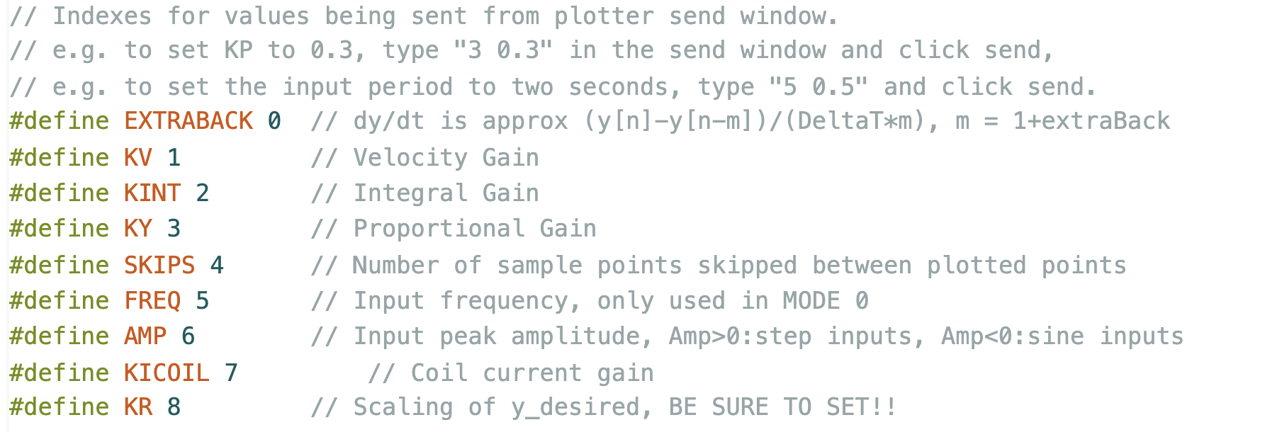
Serial Plotter Send Window Indices
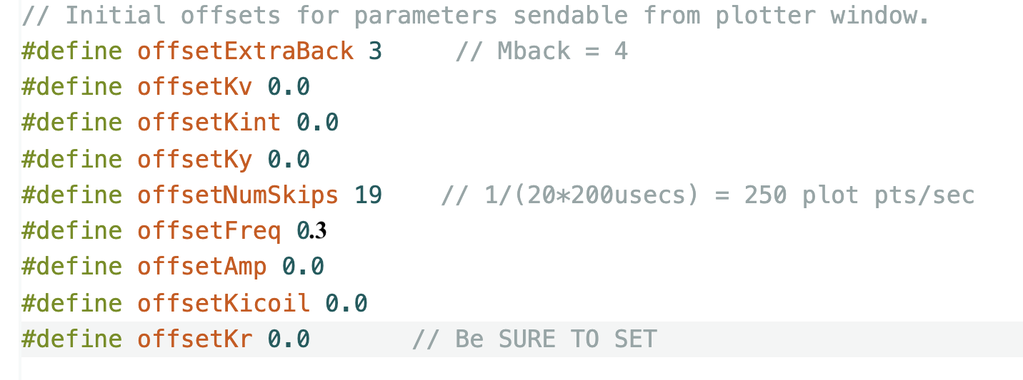
Useful Offsets to Set
Links
PLEASE USE YOUR PYTHON SCRIPT AND TEENSY SKETCH FROM LAB 5!
Introduction
Please DO NOT START THIS LAB until you finished lab5b, Checkoff 5. That is, you should have a python program with a calibrated state-space model, including a position error integrator, that designs an effective controller using LQR.
If you examine your controller in action, it probably behaves like the video on the left, in which the commands generated by the Teensy microcontroller (plotted in pink) are extremely noisy when the umbrella is nearest the optical sensor. A controller designed using the approach below is shown on the right, where you can clearly see that the command noise is much lower.
We fibbed when we claimed that the lab5 maglev controllers were "measured state" controllers. In fact, we were only
A Different set of states.
In lab4a and lab4b, we started with the transfer function relating Teensy command to umbrella position,
In lab4, our controllers only fed back back measured umbrella position, but for state-space controllers in lab5, we wanted to feed back measured coil current, measured umbrella position, and measured umbrella velocity. We factored \gamma from the above H(s) into a product, as in \gamma = \gamma_{di/dc}\gamma_{da/di}, and determined the factors by measuring coil-current (along with umbrella position) in closed-loop step responses. In the resulting transfer function,
Suppose instead we wrote the Teensy command to umbrella position transfer function in a form that was easy to factor into a product of three transfer functions,
There is only one check-off in this lab. You should be prepared to: show us your new controller (a four-state controller please: coil current, your velocity replacement, umbrella position, and the integral of the position error), show us that using the new controller lowers command noise, and explain to us how you designed your controller. Please start with your integral controller python script and Teensy sketch from the last checkoff of lab 5, and modify them to use the new state estimate.
If you are not sure how to get started, we have some suggestions below, but as always, please, please, please ask for help if you are stuck.
Some Suggestions and Hints.
Hints
- Which is likely to be less noisy, an estimate based on integrating (numerically) the measured coil current, or an estimate based on differentiating (again numerically) the measured umbrella position?
- If your new state satisfies a differential equation, should that equation be stable or unstable?
- To implement the lead controller in lab4b, you turned a transfer function into a differential equation, and then discretized the differential equation on the Teensy. Reviewing how the discretized differential equation was implemented on a Teensy might help you with the implementation for this lab.
Suggestions
- USE a four-state model, including the integral of the position error!!
- Use FIVE pins and a little disc magnet on the umbrella to minimize rocking!
- After you have a working controller, you may notice that the controller magnifies umbrella rocking. There are several ways to mitigate this problem.
- Rocking is magnified if \gamma_{da/dy} is underestimated. Try increasing \gamma_{da/dy} by fifty percent, redesign your controller, and see if the sensitivity to rocking improves.
- Try adjusting the current scaling in your model and redesigning the controller. Avoid increases by more than fifty percent.
- Try adjusting the LQR weights to minimize the gain (the K) applied to the estimated state.
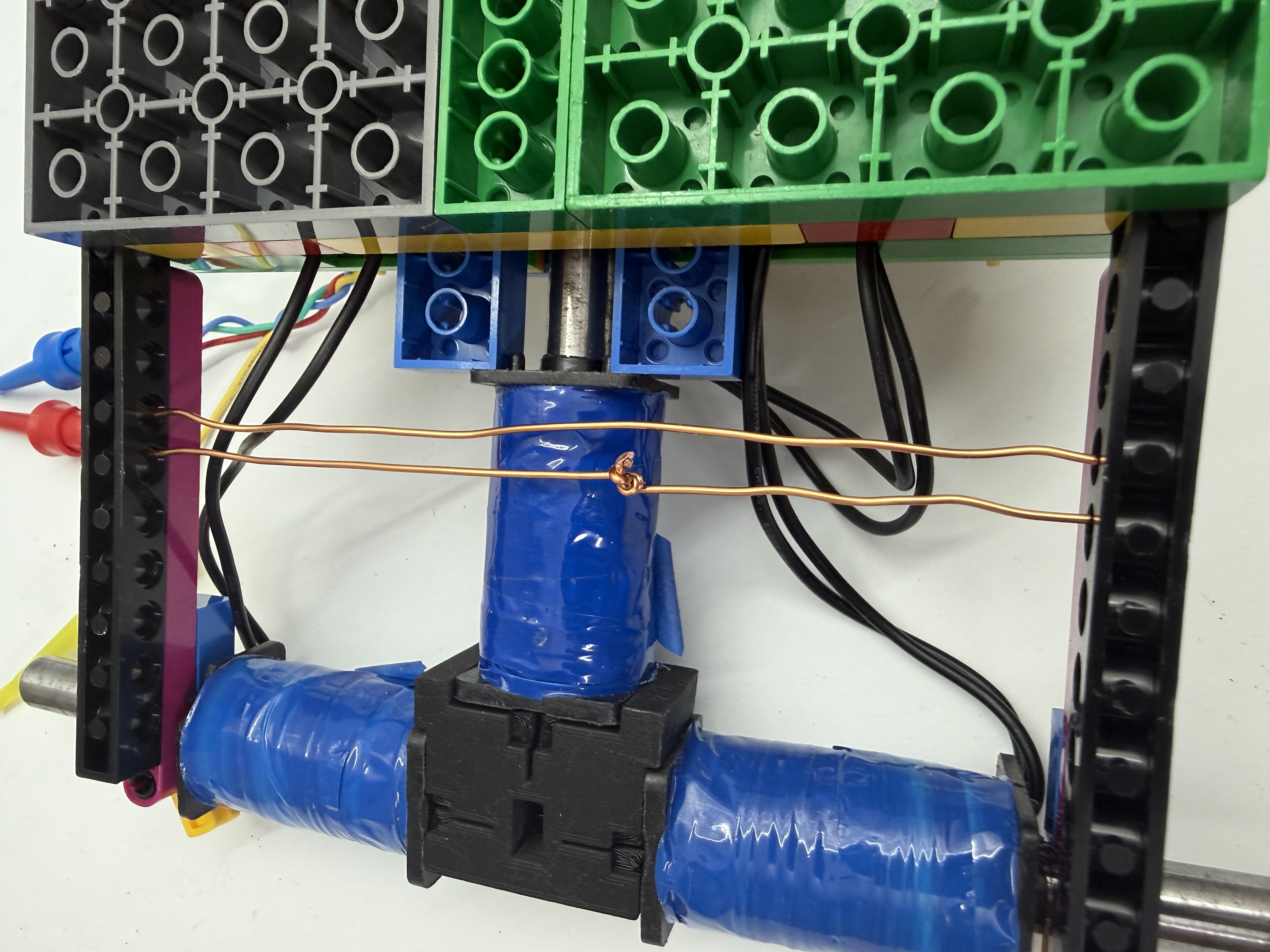
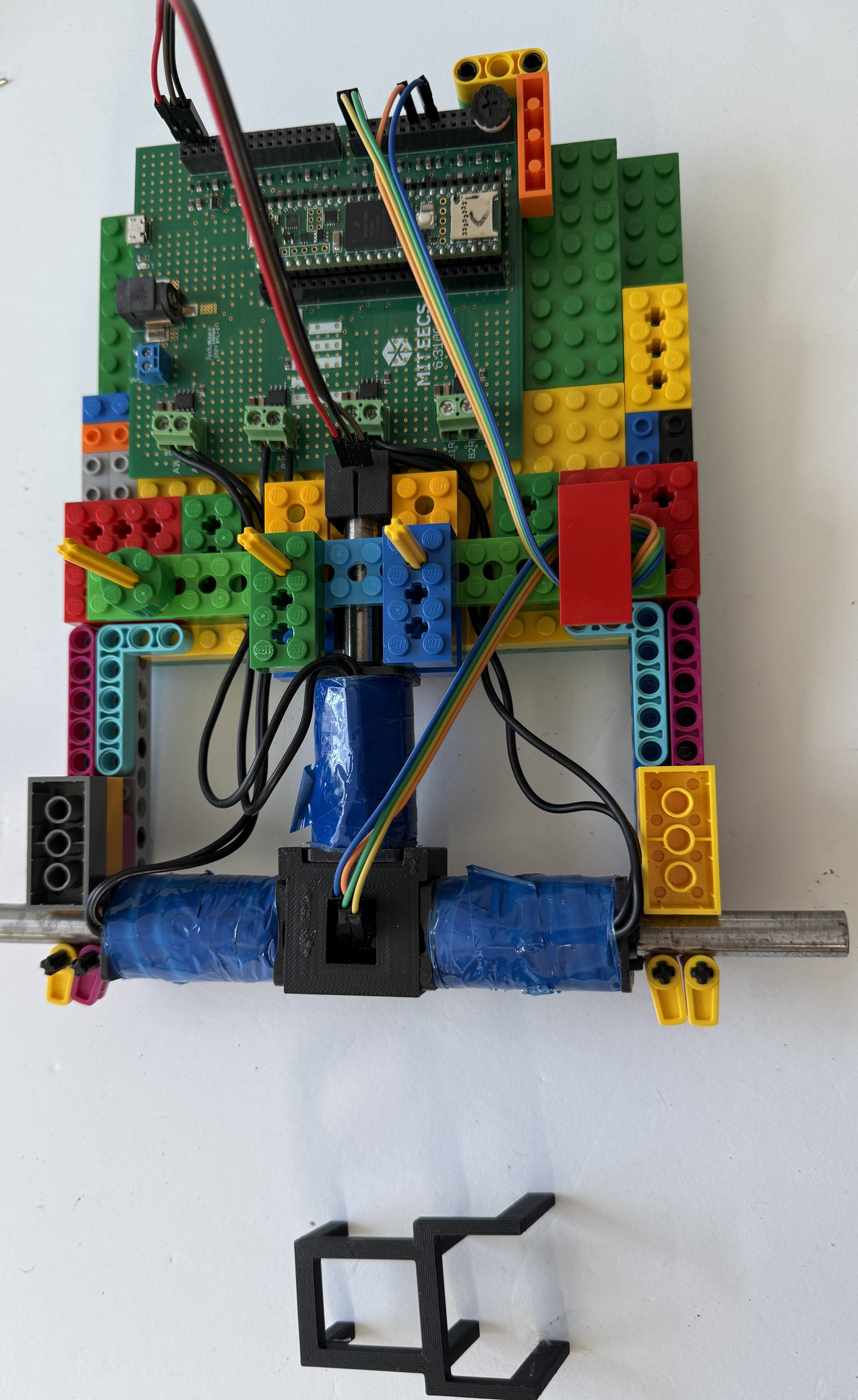
- The maglev setups get warm enough to soften PLA, causing the brackets to "droop." We have a range of suggestions to help with that. You can add a guy wire (left image below) or we can help you build a heavier-duty version (right image below).
The checkoff.
Please be sure you are ready to describe your python design code and your Teensy implementation.
Integral Controller
