Lab 6:
Observe and Learn
Please Log In for full access to the web site.
Note that this link will take you to an external site (https://shimmer.mit.edu) to authenticate, and then you will be redirected back to this page.
Serial Plotter Send Window Indices
| EXTRABACK 0 | dx/dt is approx (x[n]-x[n-m])/(DeltaT*m), m = 1+extraBack |
| KD 1 | Derivative Gain |
| KP 3 | Proportional Gain |
| SKIPS 4 | Number of sample points skipped between plotted points |
| FREQ 5 | Input frequency, only used in MODE 1 |
| AMP 6 | Input amplitude for square wave (if > 0) or sine (if < 0) |
| EST 7 | Use estimated state if > 0, measured state if < 0. |
Useful Offsets to Set
| offsetExtraBack 20 | 20 is very high, used to reduced noise and make plots interpretable. | |
| offsetKd 0.06 | Low gains for model fitting sweep | |
| offsetKp 0.5 | Low gian for model fitting sweep | |
| offsetNumSkips 4 | plot point every 5 samples, 5*2ms=10ms, or 100 points per second. | |
| offsetAmp 0.15 | Input togggles between -0.15 and 0.15 radians in sweeper. | |
| offsetEstState 1 | Positive, so use estimated state | |
Links
- All files for this lab (Teensy sketch + Python scripts) are in one zip here.
- Please reassemble the two-propeller arm using the simplified assembly described below.
- Python dependencies: this lab requires a number of python toolboxes:
numpy,scipy,matplotlib,pyserial,control.
Introduction
For this lab, you will use a regression-based strategy to "learn" a state-space model directly from frequency response data, and then use this model to design an observer-based state-space controller. Specifically, you will:
- rebuild the two-propeller arm,
- run the Teensy sketch in frequency sweeper mode to measure the arm's frequency response,
- fit a state-space model to the propeller arm frequency response,
- determine weights for LQR and then use it to compute gains for an observer-based state-space controller,
- upload your controller to your two-propeller arm, and use your measurements to further optimize the LQR weights.
A Few Examples
The above strategy is quite effective, and remarkably robust once the LQR weights are determined thoughtfully, as we show in the three videos below. In each video, the propeller arm is using a controller generated by the above strategy, and is reacting to desired-angle step changes of +/- one hundred degrees. The first video shows the poor performance of the propeller arm with the controller generated by the default LQR weights in the Python script we provided, the second shows a pretty good controller generated by improving the LQR weights, and the third video shows very similar good performance on an arm with FOUR motors without ANY software changes, just rerunning the sweeper to re-measure the frequency response.
In the leftmost video above, the arm uses the default controller. Notice that the estimated arm velocity, plotted in pink on the computer screen, separates from the measured velocity, plotted in blue, during arm transitions. Note also that the arm overshoots the desired angle significantly, and settles very slowly. In the middle video, the arm uses a controller generated by optimizing the weights. Notice how well the state estimates track the measured states and the limited overshoot. Notice also, the arm's resilience to tapping disturbances. The rightmost video shows an arm with four motors behaving very similarly to the two-motor arm in the second. Exactly the same software that generated the controller for the two-motor arm was used to generate the four-motor arm controller (frequency sweeper, model extractor, LQR weights, etc). That is, the extracted model and controller gains were not the same, but the algorithms to compute them were identical.
Expect to do better
After you've fit your arm with a model, and used the simulation tools to help you determine how to best modify the LQR weights, you should be able to design an observer-based controller that out-performs the pretty-good controller above. In particular, see how close you can get to a rotation step near the sensor limit of +/- 160 degrees. To do that, you will need a controller with far less overshoot than the "pretty good" examples above.
Learning to Model
In all the past labs, we have designed feedback controllers by first developing a model of our system, and then using that model to determine a good controller. As we moved from proportional to PID to Lead-Lag to State-Feedback controllers, we needed progressively more comprehensive models to design these progressively more sophisticated controllers. Unfortunately, our approach to modeling has NOT become more sophisticated. We continue to rely on ad-hoc combinations of physical insight, simplifying assumptions, and measurements.
Until now.
Please use the simplified assembly instructions below to reassemble the propeller arm, and then download and install the software for this lab. When installed correctly, the software allows you to run the Teensy sketch in frequency sweeper mode; capture your arm frequency response in a file (sweeper.csv); fit the frequency response with a state-space model; use the state-space model to design an observer-based state-space controller; simulate the performance of the controller; upload the controller to the Teensy; and test your controller's performance on your propeller arm. You will also be able to change your controller design in Python, WITHOUT RERUNNING THE SWEEPER, and by rerunning the Python script and then re-uploading the Teensy sketch, automatically upload the updated controller. The controller will automatically transfer from Python to the Teensy sketch, no copy and paste required!
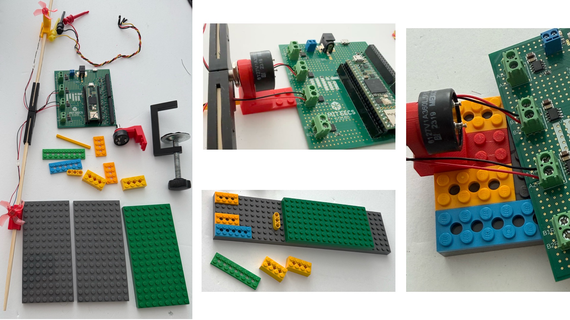
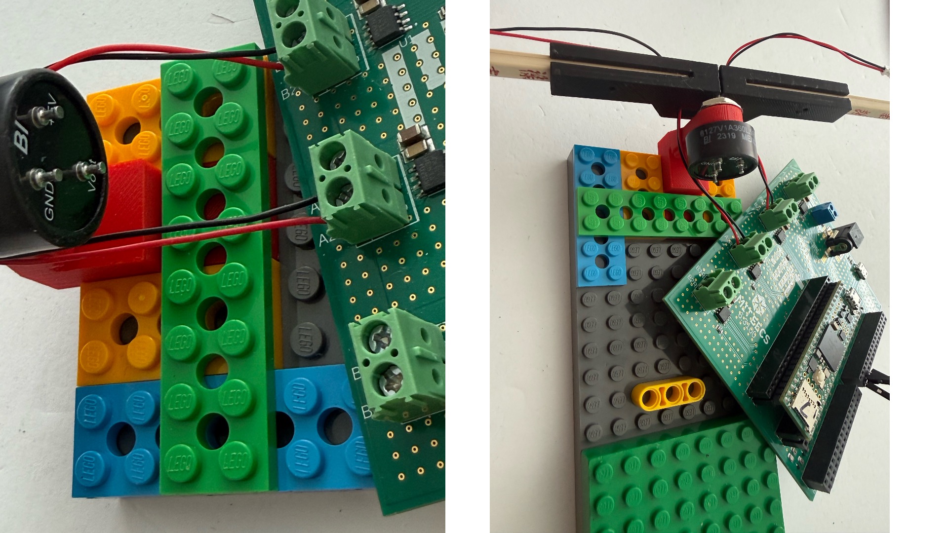
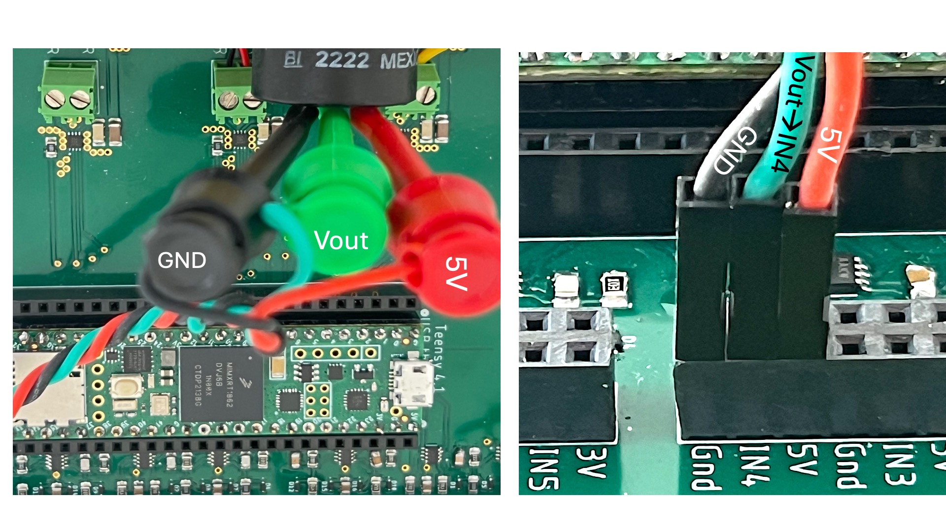
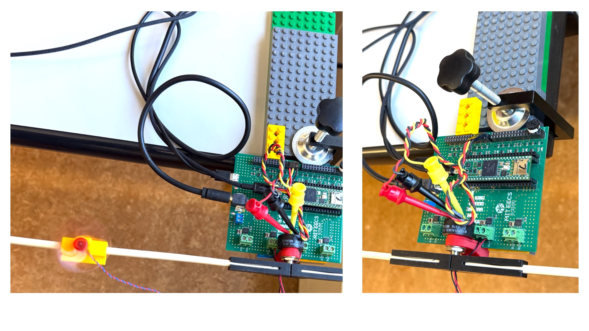
Simplified Arm Reassembly
In the five following images, we show how to quickly reassemble the propeller arm.
Software Setup
The Python scripts and the Teensy sketch to support this lab are all in one zip file, linked on the top of this page. Please download the zip file, but DO NOT UNZIP THE FILE!!!
Make sure you have a recent Python (3.9+) installed. Open a terminal (Terminal on macOS/Linux, PowerShell on Windows) and install the lab's dependencies:
python -m pip install numpy scipy matplotlib pyserial control
(If you have both python2 and python3 installed, use python3 -m pip ... instead.) The control package is the python-control library and provides the lqr, dlqr, place, ss, tf, and Bode-plot routines we use in place of MATLAB's Control System Toolbox.
Create a course6310 folder in a directory THAT IS LOCAL TO YOUR COMPUTER. DO NOT create the folder in any iCloud directory (MAC), or oneDrive, or Dropbox, or .... These services do not guarantee sufficiently quick file updates, and can interfere with the automatic updating of your controller.
Please move the downloaded zip file to the course6310 directory you just created and, ONLY THEN, unzip the file into a subdirectory. Unzipping the file should create a 6310_CT_PROP_OBS_SWEEP_26 subsubdirectory which contains this lab's files: the Teensy sketch, 6310_CT_PROP_OBS_SWEEP_26.ino; a main Python script file, prop26SS.py ; five Python helper modules (labFitter.py, simMsfObsf.py, plotSys.py, synthData.py, printTeensyObserver.py); a Python sweeper-capture program csvGen26.py, which captures sweeper data into a CSV file; and two program-generated files, sweep.csv and obs6310.h. The sweep.csv file is generated by csvGen26.py, and is read by the Python script. The obs6310.h file is generated by the Python script, and read when the 6310_CT_PROP_OBS_SWEEP_26.ino file is compiled and uploaded to the Teensy.
Open a terminal in the 6310_CT_PROP_OBS_SWEEP_26 directory and run python prop26SS.py (or python3 prop26SS.py). Open the 6310_CT_PROP_OBS_SWEEP_26.ino sketch in the Arduino IDE (both files should be in exactly the same directory). If the software is set up correctly, running prop26SS.py updates your local copy of obs6310.h. Then when you compile and upload the Teensy sketch you opened, it picks up the freshly written obs6310.h file.
Checkoff 1
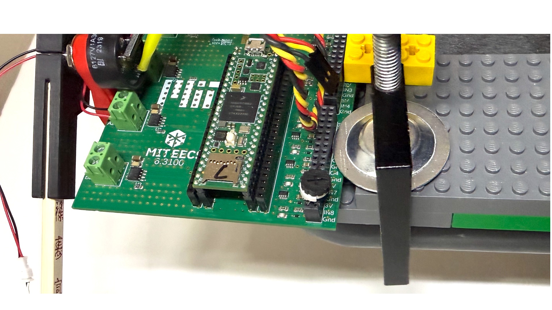
Please reassemble the simplified propellor arm as shown in the figures below, and then use the 6310_CT_PROP_OBS_SWEEP_26.ino sketch, with MODE set to 0 (on line 13), recalibrate the angle sensor so the angle is zero when the arm is level and set the motor directions so that both motors blow downward (the AngleOffset is on line 14 and the hbridgeBipolar commands are on near line 375).

Measuring Frequency Response
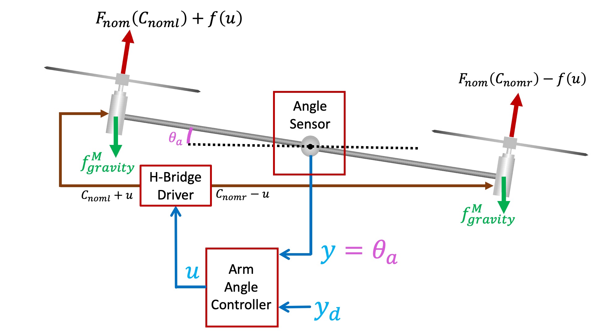
Recall that when we last encountered the propeller arm, we started with a functional diagram of the arm, shown below.
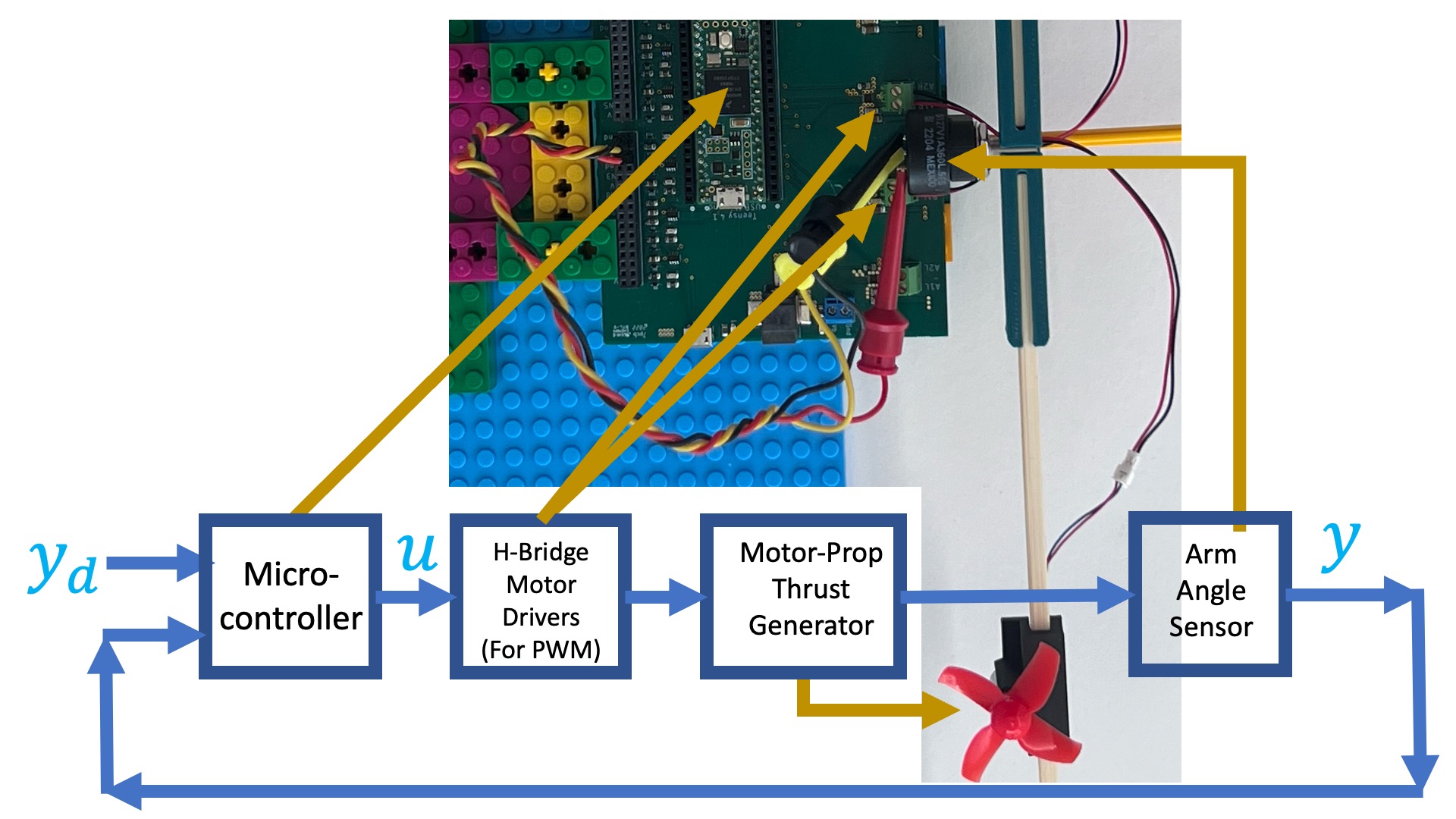
If we are interested in measuring arm frequency response, we can stabilize the arm with a controller. For the stabilized arm, we can set the desired angle to a sinusoid y_d(t) = sin(2\pi ft) = sin(\omega t). If we wait long enough, then the output of the controller, u(t), and the measured arm angle, y(t), will be sinusoids of exactly the same frequency as the desired angle but not exactly the same amplitudes and phases. We can then use the amplitude ratios and phase differences to compute the propeller arm transfer function H(j\omega).
In the control system diagram below, we show the software blocks to clarify the fact that the controller output u is explicitly generated in the Teensy sketch, and that the arm angle, y, is explicitly measured. As a result, we can easily record the magnitudes and phases (or equivalently, real and imaginary amplitudes) of u(t) and y(t).
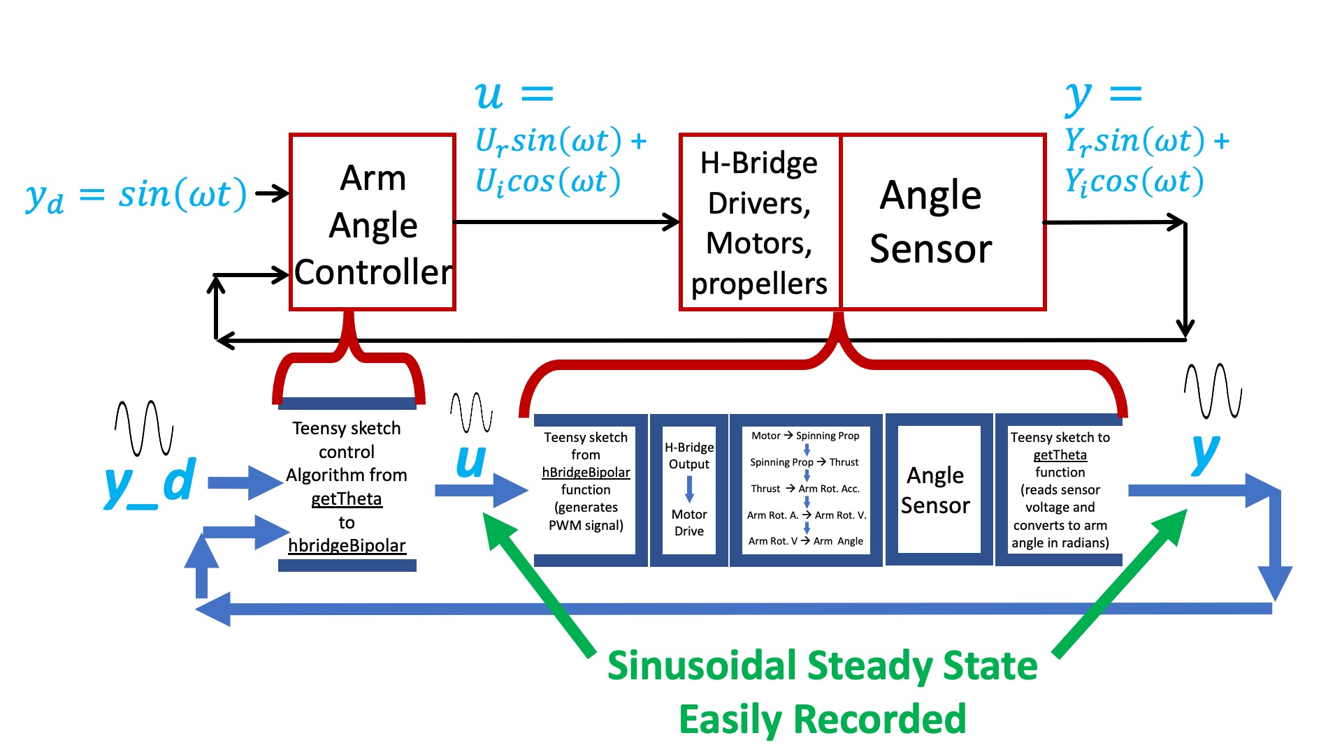
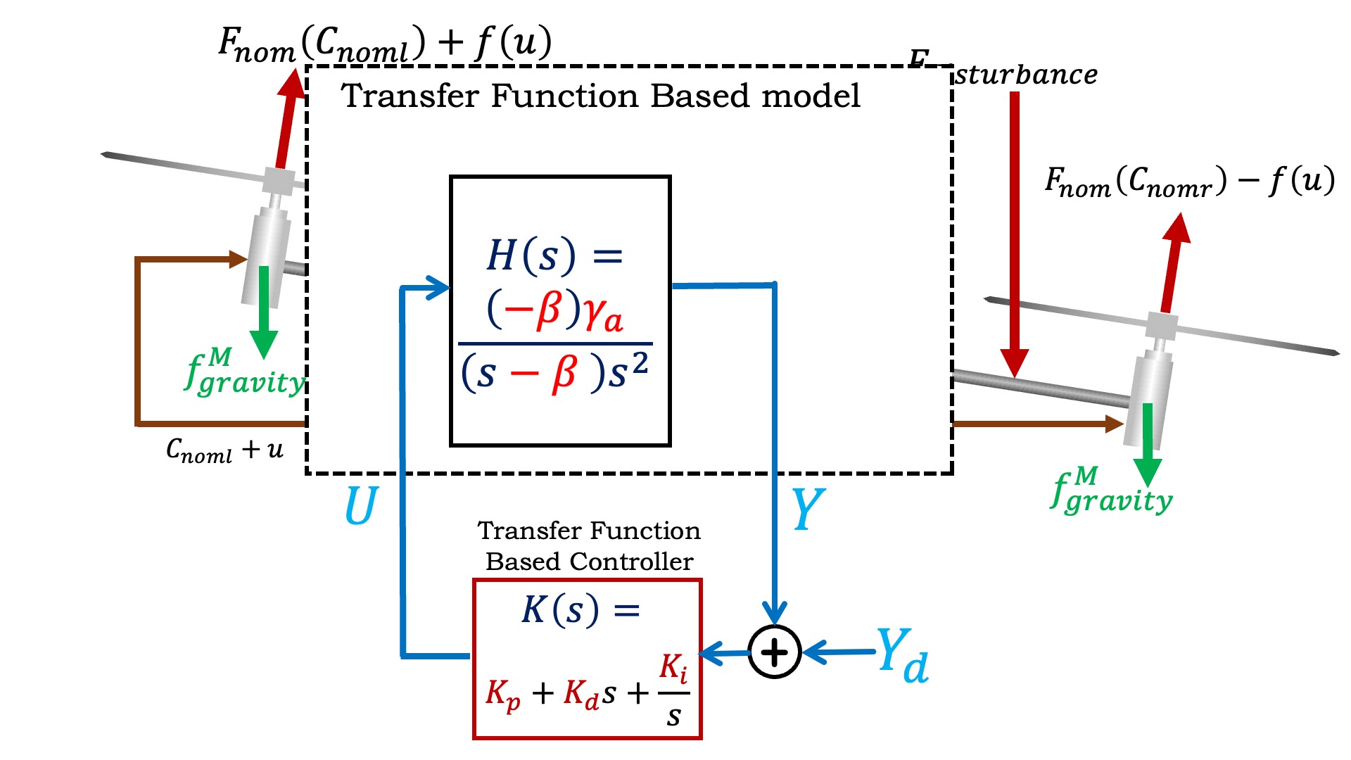
Given the measured sinusoidal steady state amplitudes and phases (or equivalently, real and imaginary parts) for both the command to the arm and the measured arm angle, it is easy to de-embed the arm frequency response from the response of the control system as a whole, as shown below.
Based on our previous modeling of the arm, we determined that its transfer function is of the form
You will be using a Python fitter (in labFitter.py) that approximates H(s) from frequency response data using an approach similar to the one you used in one of the previous postlabs (although the fitter also introduces additional constraints to favor a more physically reasonable result — here the SciPy invfreqs routine, weighted to favor moderate-magnitude points). As we noted in the last lab, transfer functions do not uniquely define state-space representations. You will have to examine the state-space matrices generated by labFitter to determine how it assigned the states.
Running the sweeper
After you have calibrated your arm, please set the MODE on line 15 in the Teensy sketch to -1, make sure both power supplies and your laptop are connected to the controller board, and then
- Open a terminal or powershell window in the 6310_CT_PROP_OBS_SWEEP_26 subdirectory, and try typing "python csvGen26.py" (or python3 if you have both python2 and python3 installed) in that window. If you do not get an error in a couple of seconds, type control-C in the window to stop the program.
- If you got an error like "serial.tools....not found..", type "python -m pip install pyserial" followed by return in the command window. If you get an error associated with matplotlib, type "python -m pip install matplotlib". If you are using python3, type the above commands, but substitute python3 for python.
- Upload the sketch (with MODE set to -1) onto the Teensy, close the serial plotter if it is open, and then open the serial MONITOR by clicking the circular icon at rightmost top of the arduino IDE window.
- You should see you arm oscillating and after about twenty seconds, you should see a set of numbers in the arduino monitor window.
- CLOSE THE SERIAL MONITOR WINDOW.
- Type "python csvGen26.py" or "python3 csvGen26.py" followed by return in the terminal window, and you should see numbers start to appear (like in the video below). It can take ten seconds or more for the first numbers to appear.
- Let the sweeper run through its forty frequency points at least twice (should take less than 10 minutes). Then type control-C to stop the python program.
- Sometimes the above strategy fails, and the python program never prints any numbers. Be sure that the serial plotter is NOT OPEN, then try, WITHOUT QUITTING THE PYTHON PROGRAM, reopening the Teensy serial monitor, waiting until numbers are printed, then reclose the serial monitor. That may be enough for the Arduino to "release" the USB receiver so that the python program can connect. If that does not work, quit everything (Arduino, Teensy and python), and try again.
- Run
python prop26SS.py(orpython3 prop26SS.py) in the same directory; it should pick up the recorded frequency response and create a model.
The video below shows the sweeper sweeping (using a PREVIOUS TERM's setup!).
After the Python script fits the model, you should be able to inspect the matrices A, B, and C in the Python session (e.g. start the script with python -i prop26SS.py to drop into an interactive prompt at the end), and see reasonable values.
Checkoff 2
Run the sweeper, collect the sweep data as described above, and generate the state-space model.
nPoles and nZeros near the top of prop26SS.py). Explain the reasoning behind this assumption.h_resp = y_resp / u_resp step of labFitter.py? How will the result be used to generate a model of the propeller arm?
Observer Estimate
For the maglev system, we could directly measure the states of the system, thanks to a combination of the optical distance and the hall-effect field sensors. For the propeller arm, this is not the case. Differencing angle sensor readings is a noisy way to estimate arm velocity, and measuring propeller thrust is even more problematic. Instead, since we used a frequency sweeper and fitter to generate an accurate model for the arm, we will use simulation of that model, with angle measurement corrections, to estimate the equivalent of the arm's velocity and the net thrust.
TF Modeling and PID Control Review
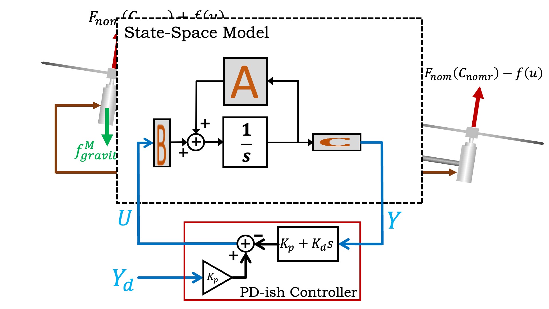
To transition from transfer function to state space modeling and control, consider the "schematic" diagram of the arm and controller, shown below.
We used physical insight to uncover a transfer function description of the propeller arm, used measurements to calibrate the model, and examined pole locations and disturbance transfer functions to determine good PID controller gains.
State-space and Observer-based Control
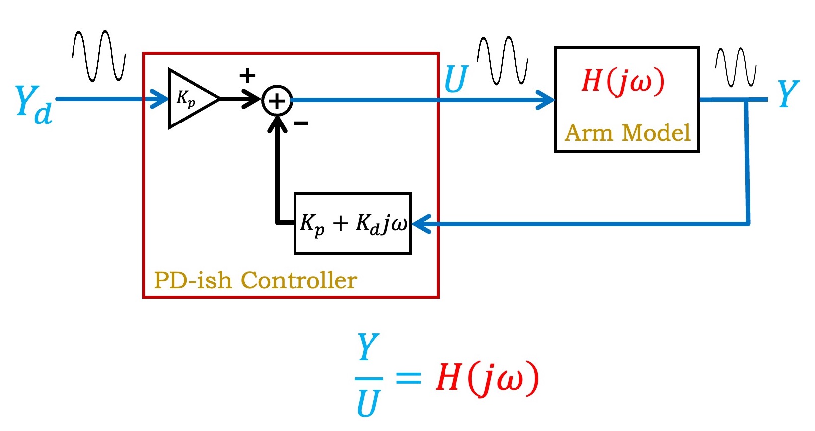
We can replace the transfer function model of the arm with a state-space model, as shown in the figure below. Also shown in the figure is the PD-ish controller that was used to stabilize the arm, which made it possible to measure the unstable arm's frequency response.
Since you synthesized a state-space model from frequency response measurements of your particular arm, you can expect that your model is accurate. And given an accurate state-space model for the arm, you can use it to generate an observer. The observer time-evolves a simulation of the state-space model, with corrections based on comparing predicted and measured outputs (angles in this case). These continuously-corrected estimated states are then used for estimated-state feedback, as show below.
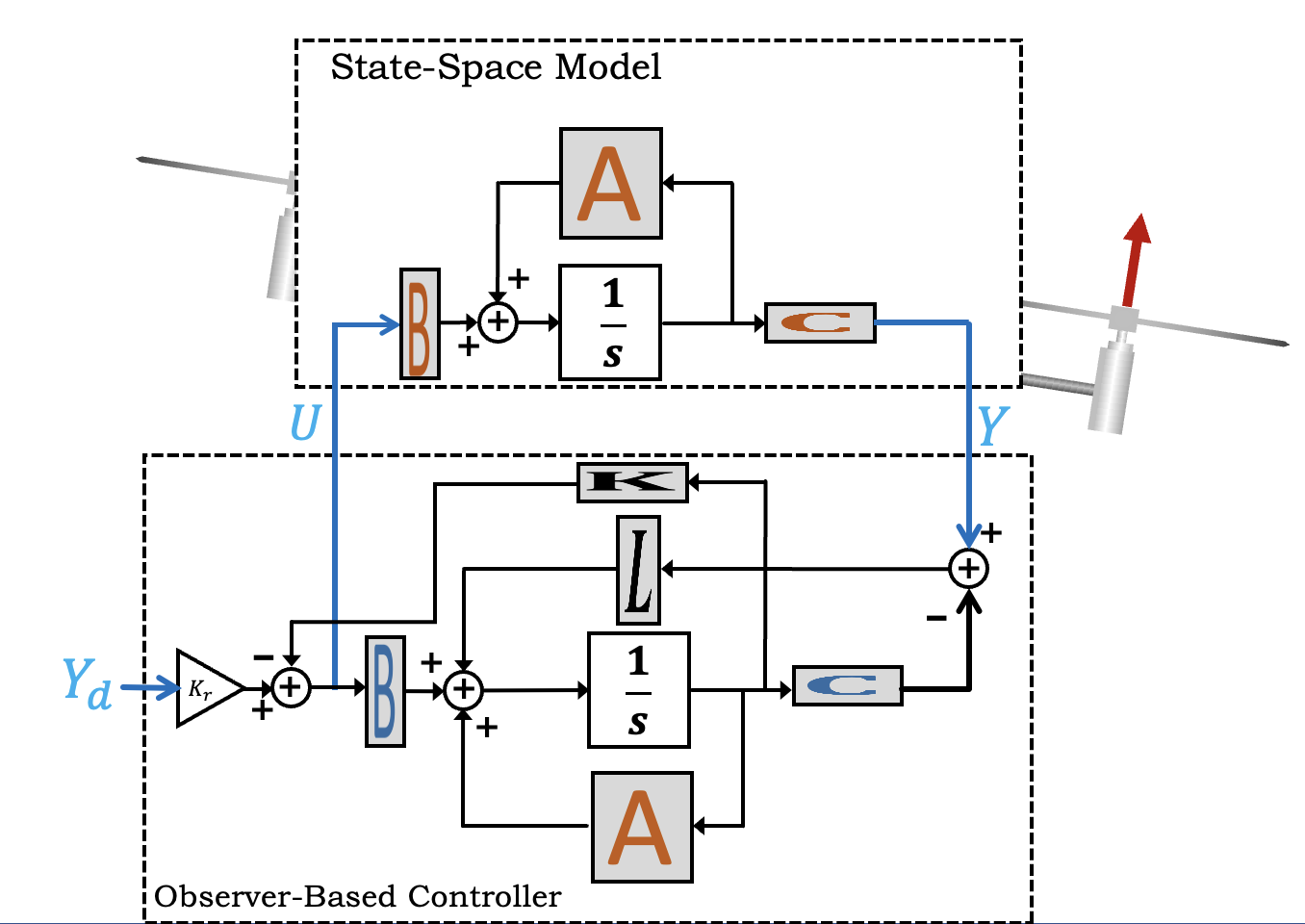
As the above figure makes clear, when we use an observer-based state-feedback controller, we have two sets of gains to determine. The first are the state-feedback gains summarized in the vector K, and we know how to use LQR to determine K. The second set of gains are the observer (or state-correction) gains, summarized in the vector L, and these can also be determined using LQR.
When using LQR to determine state-feedback gains, one sets relative state weights (Q) by determining which states should go to zero fastest, and the relative control weight (R) based on ensuring the commands do not become too large. When using LQR to determine observer gains, the approach to setting weights is not as obvious, and we will return to the issue in part B of this lab.
Pole-Placement Based Observer
Using a state-space controller and an observer-based state estimator requires two sets of gains, controller gains (the K's), and estimator correction gains (the L's), and we will need insight into how to select those gains. In lecture we learned that the poles of the control system are eigenvalues of A-BK, and poles of the estimation error system are the eigenvalues of A-LC, so we can compare the two sets of poles to see if the estimation error is converging much more slowly than the controller. But what is too slow? And for systems with multiple poles, how should we compare?
Run the prop26SS.py script, examine the plots it produces and the output it prints.
Checkoff 3: Examining the Default Controller
END OF ASSIGNMENT FOR WEEK A
Checkoff 4: Mind your K's and L's.
Use what you've learned in the previous lab and adjust the LQR weights for the controller in prop26SS.py (the Q and R assignments in the "CT Measured-State Feedback" section), and use what you have learned about DT observers to optimize the place call (the obs_poles list in the "Observer gains" section). Examine the simulation results as you make adjustments, to see how your changes effect propeller behavior (e.g. overshoot), disturbance rejection, and estimation accuracy. Once satisfied with the simulation results, test your controller on the arm using smaller step-sizes, +/- thirty degrees or less. Try to minimize the command noise without compromising performance by iterating between Python, examining simulation, and the Teensy experiments, and examining step responses. You should end up with a MUCH BETTER controller!!!
Checkoff 5: Out for a Spin?
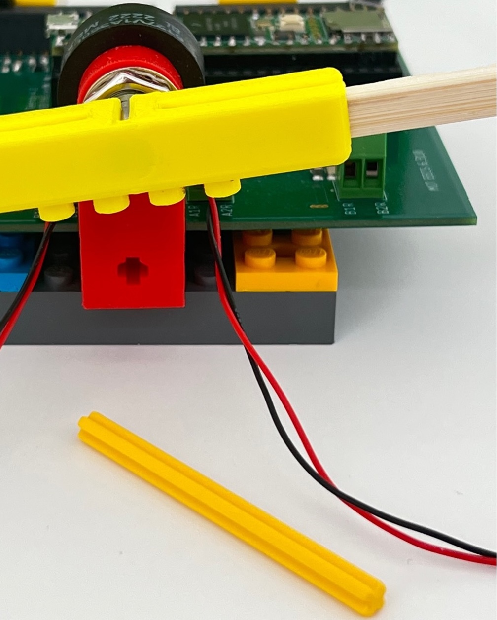
If you remove the rotation-limiting cross piece, as in the figure below, you can take much larger steps.
When you try larger step-sizes you should notice a problem with the estimated states. Check lines 360->374 in the Teensy sketch. Is the u controlling the arm EXACTLY the same as the u used in the observer?
Once you have fixed the Teensy sketch, do you get better matches between the estimated and measured states? If so, try to find controller gains for which large angle steps do NOT overshoot. Then see how close you can get to the maximum rotation angle step (about +/-170 degrees).
How did you avoid overshoot?
Checkoff Six: Pack Up!
A Fitting End with a Nagging Question.
After you complete this lab, you might think that the fitting approach works so well, and seems so automatic, that maybe you did not need all of the material we covered in 6.310. If you are having such second thoughts, please think about using the approach for a completely new problem.
You'll have to decide what to actuate and what to sense. And since you can only measure frequency response if your system is stable and nearly linear, you will have to decide how to linearize and stabilize your system. And if you stabilize your system with a classical controller, you will have to determine how to de-embed the controller from the measured frequency response. How many frequencies should you measure, and over what range? And how will you "regularize" the fitter? And once you generate the model, how will you determine the LQR weights for the controller and the estimator? What experiments will you try?
Oh and one last nagging question. Consider the relationship between \hat{y_f}, the feedback contribution to the controller output u, and the y's, the entire past history of measured angles. Abstractly, the observer-based controller is summarizing all the past measurements with a few internal states, and is then updating u with a weighted combination of those states. Maybe we could pick better states? Or fewer states? Maybe we could determine (or learn) better ways to update the state, and better weights to use when determining u? Statistical estimation, model-predictive control (MPC), H_2 and H_{\infty} control, and reenforcement learning (RL), are a few of the many control topics that touch on these issues, ones we did have time to cover this past term.
There is much more to the control story, and of course, many more classes to take.
Please disassemble your lab kit and return the parts to the bins located
near the center of the lab.