First Order Difference Equations
Please Log In for full access to the web site.
Note that this link will take you to an external site (https://shimmer.mit.edu) to authenticate, and then you will be redirected back to this page.
First-Order Difference and Differential Equations
In this problem we use first-order differential equations as a simple setting in which to introduce many continuous-time concepts including those you have seen before (e.g. step response and steady-state) as well as new ones (e.g. transfer functions and frequency response).
Discrete Time Reminder
As a reminder, our notation for a general first-order difference equation with input sequence u and output sequence y is
where \lambda and \gamma as real scalars and n is an integer index. The general solution can be derived by induction as is
where y[0] is a given initial condition. We also decomposed y into its zero-input response,
Aside: The input u does not have to be constant for there to be a steady-state. It is enough for u[n] = u[\infty] for n > n_0 where n_0 is a finite positive integer (u settles to a constant for n large enough).
Continuous Time Solutions
In continuous time, our notation for a general first-order differential equation with input waveform (i.e. function of time) u and output waveform y is
Aside: Since the time-derivative of e^{\lambda t} is equal to \lambda e^{\lambda t}, a scaling of the same function function, we often say that e^{\lambda t} is an eigenfunction of the differentiation operator, with eigenvalue \lambda.
We can decompose y(t) into its zero-input response,
CT Natural Frequency
Recall that in discrete time, if some non-zero y_{ZIR}[n] satisfies
In continuous time, if some non-zero y_{ZIR}(t) satisfies
For higher order difference equations, the DT natural frequencies were roots of higher-order polynomials, and therefore real equations could have complex natural frequencies. The same will be true for CT natural frequencies, they will be the roots of higher-order polynomials and can be complex. But we will return to the higher-order case later, for now, let us consider an example of proportional feedback leading to difference or differential equations.
Steady-State
If the system is stable, equivalently if the real part of \lambda < 0, then
Using Linearity and Time-Invariance
First-order differential equation have the same linearity and time-invariance (LTI) properties as their difference-equation counterparts, and we can often use these properties to quickly calculate responses. For example, we are often interested in the zero-state responses of stable systems to step changes in input, such as in
We can exploit the time-invariance properties by decomposing u(t) into a constant input, u_B(t), plus a step from a negative value to zero, u_A(t), as shown in the image below.
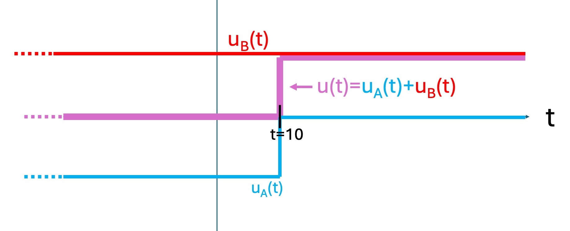
The ZSR response, given the above u(t), is then the sum of a steady-state (y[\infty] given u[\infty]=10) and a shifted ZIR response. Specifically, y(t) = 0 for t < t_0, and for t \ge t_0 is
Suppose we change the input to

Continuously Crane
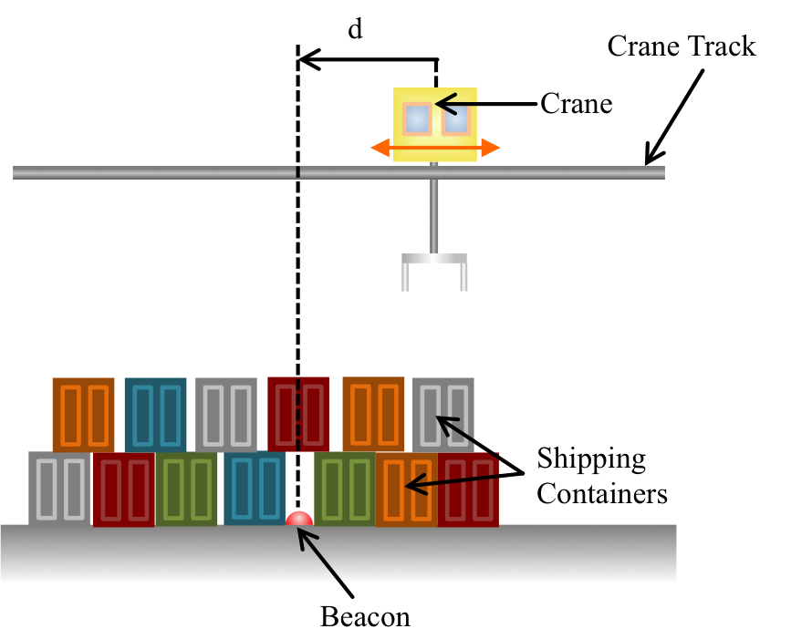
Let us return to the cargo crane traveling on track above a buried beacon, as shown in Figure 2. Suppose we must decide between two control systems, a discrete-time controller that measures distance to the beacon every \Delta T seconds, and a continuous-time controller that measures the distance continuously. One way to compare the two systems is to examine the problem of returning the crane as rapidly as possible to "home" position, that is, back to the beacon at d = 0. And for this comparison, we are going to assume that the crane has an internal feedback controller, one allows us to design a controller that senses position and controls crane velocity (as show in Figure 3 below).
Model
For our velocity-controlled crane with discrete-time sensor,
If we use proportional control to return the robot back to the beacon (d=0), then the DT controller velocity at n \Delta T is given by
For the continuous-time controller, crane distance and velocity are related by a derivative,
Inferring Parameters
Suppose the cranes are being independently monitored with remote LIDAR, which measures the distance between the crane and the beacon every ten seconds. A test was run using the CT controller with an unknown proportional gain K_p, in which two consecutive measurements from the LIDAR system (which we can denote as d(t) and d(t+10)) gave distances of 200 meters and then 10 meters between the beacon and the crane.
What was the third consecutive LIDAR measurement, d(t+20), and to within one percent, what was the controller gain, K_p?
Complex Exponential Inputs
For the zero-input case, the differential equation
If the input to the different equation is a complex exponential,
Since the differential equation is linear,
As we will see below and more generally in later sections, the function of s that "transfers" the input u to the output y is worth labeling, as in
Step Response and Parameter Estimation
If y(0) = 0 and u(t) = 1 for t \ge 0, then u(t) = 1 e^{st} for s = 0 and
A plot of the step response for \gamma = 10 and \lambda = -100 is given below. Note that the step response settles to \frac{\gamma}{-\lambda} as t \rightarrow +\infty, and has risen to about two-thirds of the steady-state at t \approx \frac{1}{-\lambda}.
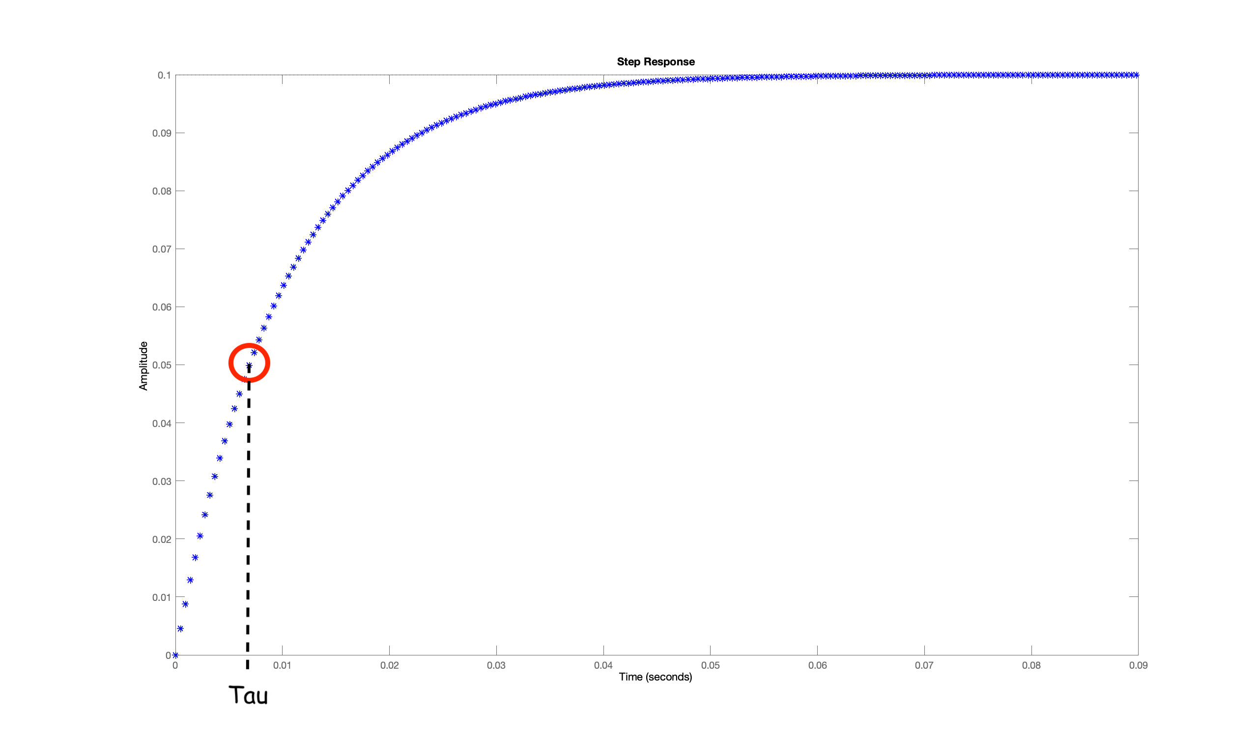
When calibrating a model using experimental data, one should design the experiments so that the needed data is both easy to measure and informative. For example, it is easy to measure the time for a step response to rise half way to steady-state (the half way point in the above figure is circled in red, and the time to rise to that halfway point is labelled Tau). Assuming the step response is well-described by the above first-order model, the half way point is given by
What model parameter can you estimate from the "half-way rise time" \tau, and what is the analytic formula for that parameter once you are given \tau? (please enter your answers as legal python expressions, using G for \gamma, L for \lambda, Tau for \tau, e**(L*t) for e^{\lambda t} and log(a) for the natural log of a (that is, log(e^a) = a).
Crane Control with Step Input
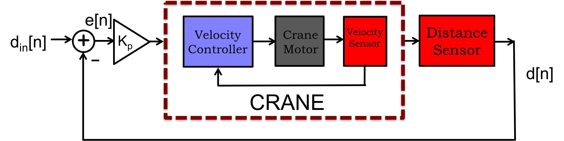
If we want to move the crane to positions other than the beacon position at d=0, we will need to specify a desired position along the track. The desired position, which we will denote as d_{in}(t), will become an input to our position controller, which will try to keep the drane position, d(t), close to the desired position d_{in}(t).
A proportional feedback approach to controlling the crane's position would be to make the crane velocity proportional to the difference between the desired and measured crane positions, as diagrammed for the DT case in the figure above. Then the velocity is given by
In order to determine how the performance of this proportional-feedback controller changes as we increase or decrease gain, we substitute the control formula in to the distance-velocity relation for the crane,
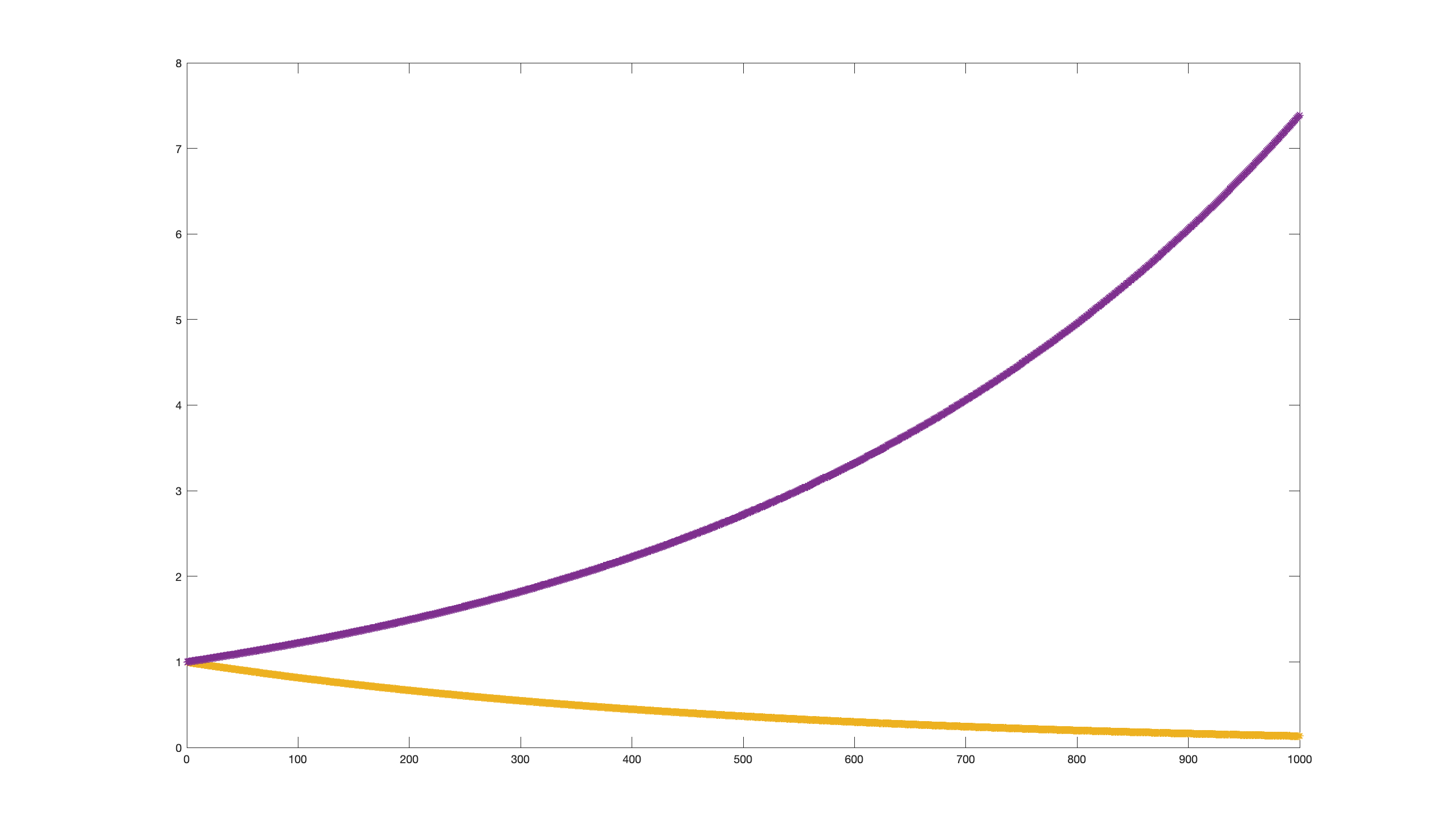
Since d_{in}(t) = 1 = e^{0t}, and d(0) = 5, we can determine the analytic solution for d(t) as a function of K_p and t (Hint: specialize the general result from the previous subsection). Use a python expression, use Kp to for K_p and use, for example, e**(-a*t) to represent e^{-at}.
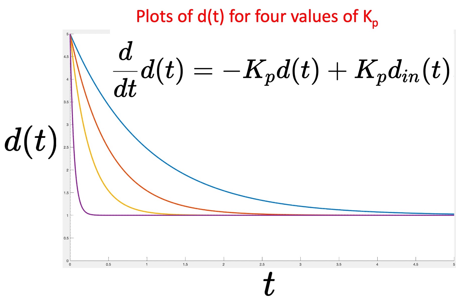
Above are four plots of d(t) versus time for the case d(0) = 5 and d_{in}(t) = 1. There are four plots, blue, orange,yellow and purple, and each plot is rassociated with a different value of K_p. Assuming that the four K_p values are integers in the range \{1,...20\}, what are the four gains in blue, orange, yellow, and purple (hint, e^{-1} \approx \frac{1}{3}). Enter your solution as a python list, e.g. [5,10,15,20].
Frequency Response
As you have already seen in lab, we can learn many characteristics of a stable system by applying sine waves to the system, waiting for the system to achieve sinusoidal steady-state, and then measuring that steady-state response. We show a diagram of that process below (note that in 6.3100 the "oscillator" and "oscilloscope" are virtual. That is, they are implemented using a combination of software, the Teensy controller board, and your laptop).
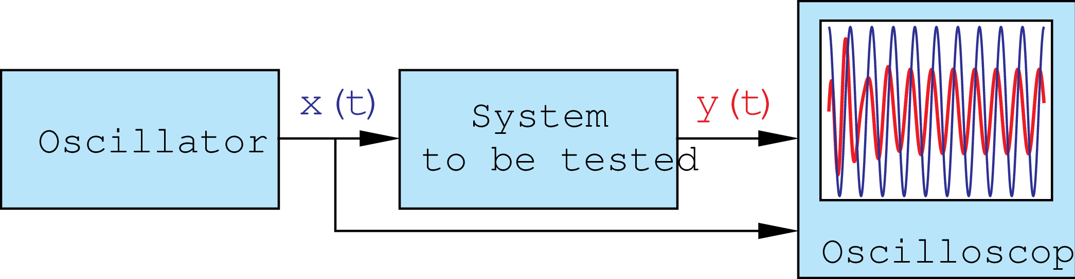
For any LTI system in sinusoidal-steady-state, the output frequency always matches the input frequency. It is the frequency-dependence of the input-output amplitude ratio and input-output phase difference, collectively referred to as the frequency response, that can reveal the specifics of an LTI system. As we will see below for the first-order differential equation case (and later more generally), we can connect the frequency response to the transfer function, H(s), mentioned above.
Sums of Complex Exponentials
We noted above that if the input, u(t), to our general first-order differential equation,
Linearity insures that we can generalize the above to inputs which are sums of complex exponentials. That is, if
If our system is stable, that is \operatorname{Re}(\lambda) < 0, and the ZIR decays faster than any of the inputs, that is \operatorname{Re}(\lambda) < \operatorname{Re}(s_k) for all s_k, then if t is large enough
There is an important class of inputs that decay more slowly than the natural response of any stable system. Sines and cosines NEVER decay, which is why they are used for system characterization.
Sines, Cosines, Magnitude and Phase.
If u(t) = Ue^{st} with U real and s = j\omega t, then
We can construct a real input, u_r(t), while retaining the exponential form by using the sum of two complex exponentials,
If our first-order differential equation is stable (\operatorname{Re}(\lambda) < 0) and the input is u_r(t), then for large enough t,
As the above equation makes clear, magnitude and angle (or phase) are the key characteristics of frequency response.
Measuring and Plotting Frequency Responses
Setting \gamma = 1 and \lambda = -1 in our first-order differential equation
For t >> 1 (so that e^{\lambda t} = e^{-1t} \approx 0) the sinusoidal steady state approximation is valid and
The process of measuring the frequency response, applying sinusoids of progressively higher frequency and measuring the associated outputs, is best visualized as a sequence of experiments, as shown below.
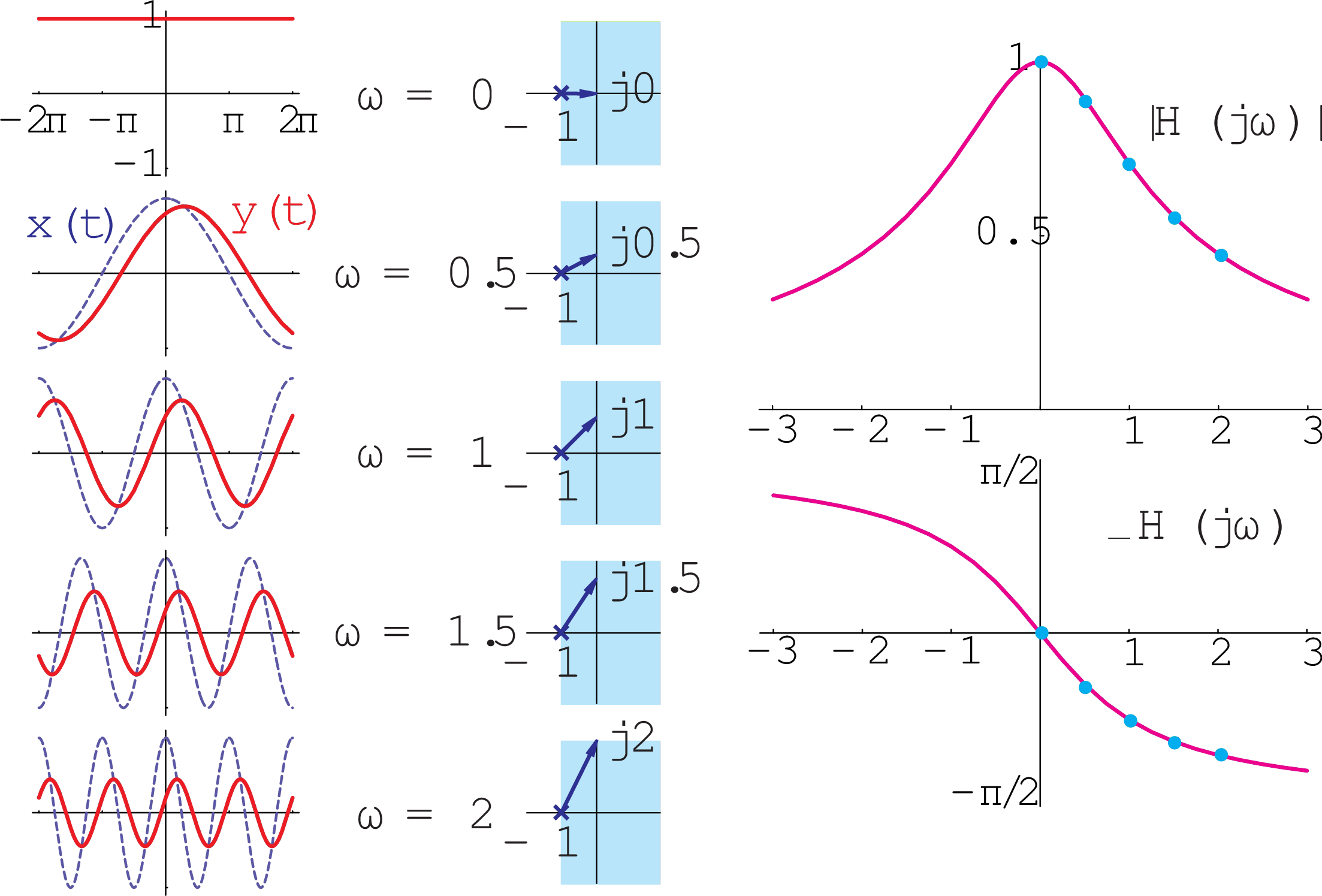
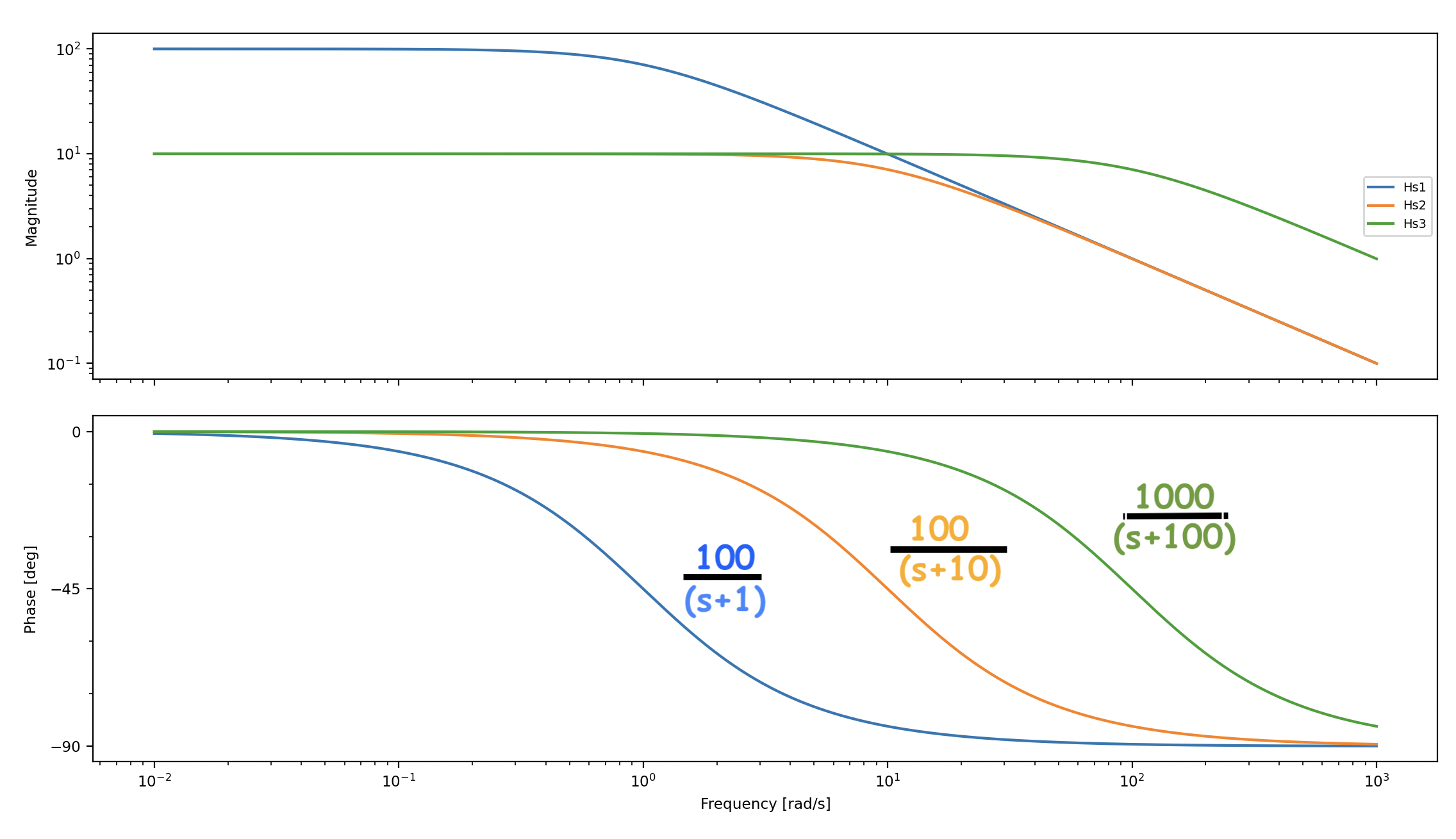
The Bode plot format,in which magnitude and phase are plotted separately and stacked, is the most common approach for plotting frequency response, or H(j\omega) versus \omega. The top plot in the Bode format is a log-log plot of |H(j\omega)| versus \omega and the bottom plot is a log-linear plot of \angle H(j\omega) (in degrees) versus \omega. Below we show Bode plots for several difference transfer functions.
Frequency Response and Parameter Estimation
Measuring the halfway-rise-time of a system's step response is helpful for model calibration because it is easy to measure, informative, and a single step-response experiment will generate the needed data. As the above diagram makes clear, measuring frequency response involves many experiments, so is likely to be more time-consuming (but is also more reliable, as you may have already seen in lab, and more generalizable, as we will see later).
Nevertheless, one might hope that the sinusoidal-steady-state response to a sinusoidal input at a well-chosen frequency might simplify the parameter estimation problem. To see an example of this, consider the graph below and please answer the questions that follow.
The graph below shows two plots, an input u(t) (in pink) and output y(t) (in blue) for a system that is accurately modeled by our general first-order differential equation model,
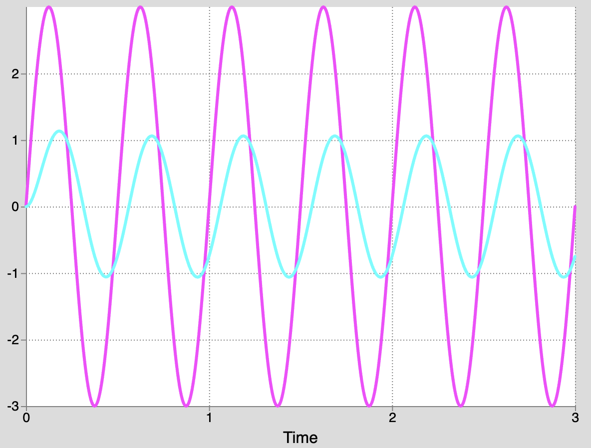
Use the graph, along with your insights about H(j\omega), to determine numerical values for \gamma and \lambda in the above model (be careful about 2*pi)!
Crane Control Frequency Response
The differential equation that describes the crane control system is given by
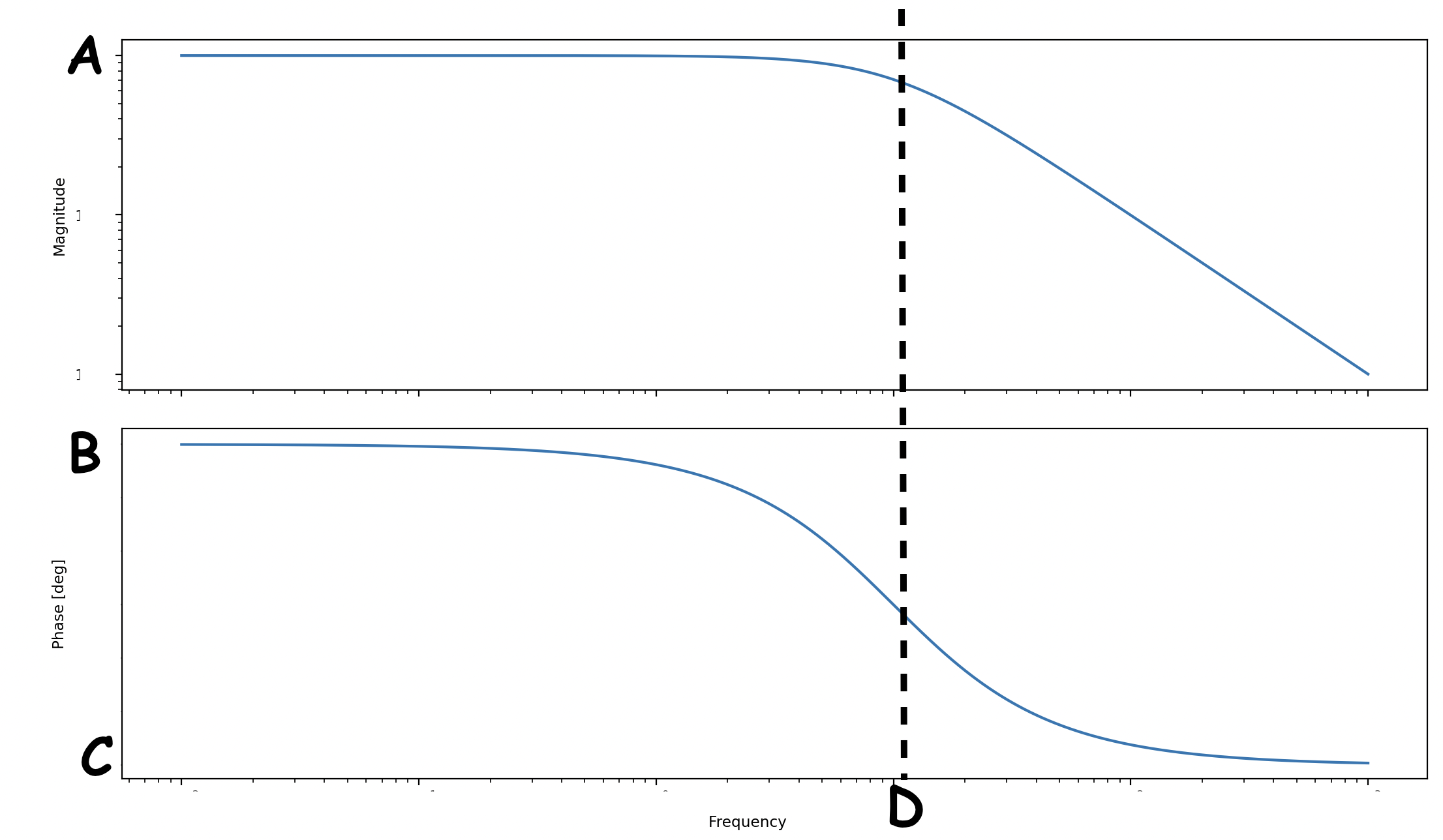
Below is a Bode-ish plot of H(j\omega), or more precisely, a log-log plot of |H(j2\pi f)| versus f, in cycles/second, and log-linear plot of \angle H(j2\pi f) (in degrees) versus f, again in cycles/second. As you can see, we have removed the axis labels, so please determine magnitude A, angle C (assume angle B=0), and frequency D (in cycles/second NOT radians/second) as functions of K_p. (Hint: only one of the labels is dependent on K_p).
In answering the questions below, use Kp for K_p and pi for \pi.