State-Space Motor Modeling

The questions below are due on Friday April 17, 2026; 10:00:00 AM.

You are not logged in.
Please Log In for full access to the web site.
Note that this link will take you to an external site (https://shimmer.mit.edu) to authenticate, and then you will be redirected back to this page.

You are viewing the PRELIMINARY 6.3100 Spring 2026 web site. Please note that information on this page may change throughout the semester, please check back frequently.

An Lmotor-Driven Arm

In this problem, we will consider an example that is similar to the propeller-levitated arm, a lego-motor-driven arm (for brevity, an Lmotor-driven arm). The similarities will make it easier for us to understand the structure of this new control problem, but differences will allow us to raise additional issues, while also giving us a chance to practice with the state-space concepts.

In earlier versions of 6.302, we rotated a heavier arm using a geared Lego motor, shown in the figure below. The figure also shows that we used two rubber bands to create an angle dependent torque on the motor (both to assist the motor when holding heavy loads, and to eliminate gear "backlash"). That angle dependent force will have a number of interesting consequences, ones that we hope will help you develop a better understanding of controller design.

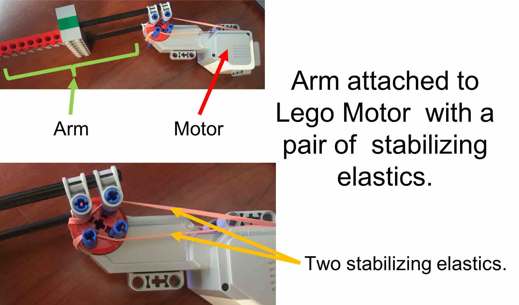
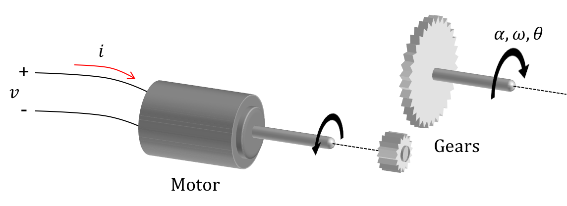
The Lmotor is a geared brushed motor, just like the propeller motor. By changing the motor voltage, v, we change the motor current, i_m, which is proportional to the torque generated by the motor. The net arm torque, a sum of motor-, gravity-, and elastic-generated torques, results in an arm rotation characterized by angular acceleration, \alpha, angular velocity, \omega, and rotation angle \theta, as shown in the figure below.

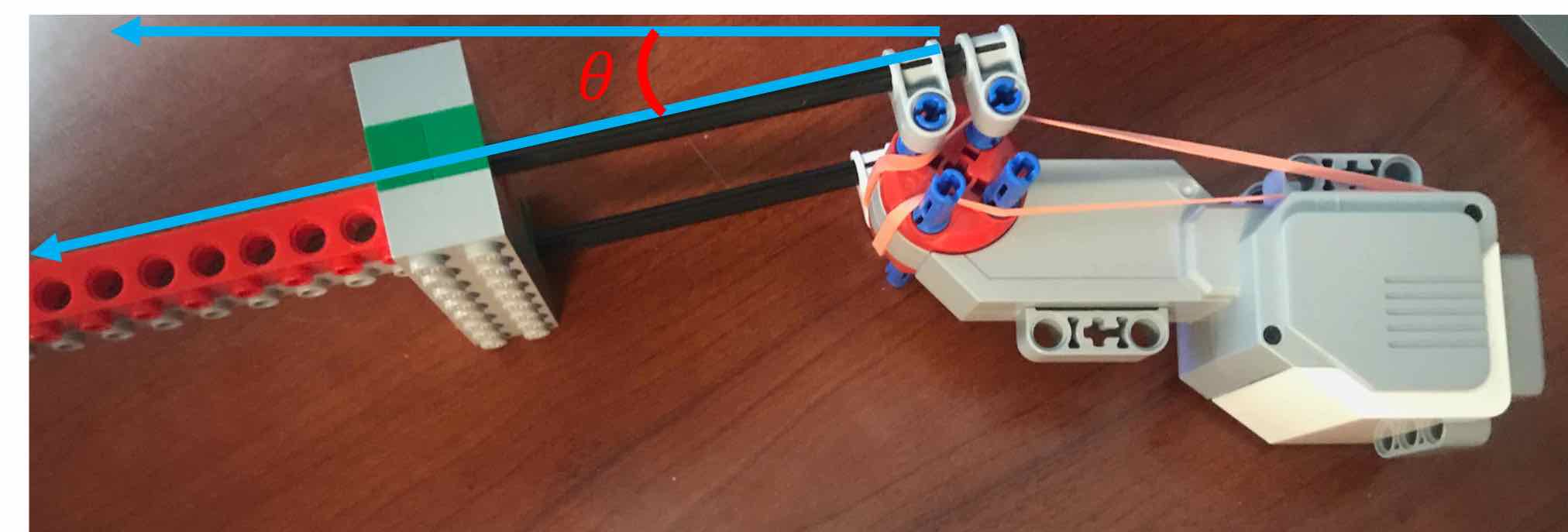
We can sense the Lmotor-driven arm angle using the same kind of angle sensor we use for the propeller arm, by linking the shaft of the angle sensor to the shaft of the motor (using heat-shrink tubing actually). As an example, using our angle sensor, we could easily measure the \theta in the figure below as approximately \frac{-\pi}{6}.

In fact, we can reuse most of our propeller-levitated arm hardware in an Lmotor-driven arm controller, since they both use brushed DC motors. We can use the same angle sensor, and we can drive the Lmotor using the same H-bridge (the Pololu board) with almost the same PWM voltages (though lego motors are designed to work with lower-frequency PWM signals). In fact, we could even use exactly the same PID controller, though we might find that good K_i, K_d, and K_p values for the Lmotor-driven arm will be different from good values for the propeller arm.

The issues in designing state-space controllers are a little different, however, as we shall see.

Generating a State-Space model

We will need a few physical relationships in order to derive a state-space model, but thankfully, the Lmotor-driven arm model does not require linearization.

The physical relationships

As in the propeller-levitated arm, the Lmotor-driven arm angle, \theta(t), is related to its angular velocity, \omega(t), through differentiation,

\frac{d \theta}{dt} = \omega(t),

and of course, the angular velocity of the arm is related to arm angular acceleration through differentiation,

\frac{d \omega(t)}{dt} = \alpha(t).

The product of the arm's moment of inertia, J, and its angular acceleration, \alpha, is equal to the torque on the arm \tau,

J \alpha(t)=\tau(t) = \tau_m(t) + \tau_b(t) + \tau_f(t),

where \tau_m is the motor-generated torque, \tau_b is the net torque generated by the rubber bands, and \tau_f is the torque due to friction. We are going to assume the arm is rotating parallel to the ground, so that we can ignore gravity as a source of torque on the arm.

As we have seen before, motor torque, \tau_m, is proportional to motor current,

\tau_m = K_m i_m,

where i_m is the motor current and K_m is the current to torque conversion factor. We can model the net torque generated by the two rubber bands as proportional to arm angle, as long as the bands have been placed so that their forces balance at \theta =0. If so, then

\tau_b = K_b \theta,

where \tau_b is the net elastic torque and K_b is the proportionality constant. Finally, the friction torque can be modeled as proportional to angular velocity,

\tau_f = -K_f \omega,

where K_f is the friction coefficient, and the negative sign is because the friction force always acts to oppose motion.

Since the Lmotor is a brushed motor, we can model it in the same way we modeled the propeller motor. That is, we can use a circuit model to relate the voltage across the motor to the current through the motor, and after scaling by K_m, relate the motor voltage to the motor torque. If we model the motor as a series combination of a motor coil resistor, R_m, a motor coil inductor, L_m, and a rotational-velocity dependent voltage source, v_{emf}, the current through the motor, i_m, can be related to the drive voltage, v, by

v(t) = R_m i_m(t) + L_m\frac{di_m(t)}{dt} + v_{emf}(t).

The motor's inductance and resistance are much larger than in the propeller motor, so the above relation can not be simplified. The v_{emf} is proportional to the motor speed, \omega_m, a fact we made use of, but did not investigate, in the SPINUP sketch used to calibrate our propeller motor.

v_{emf}(t) = K_e\omega(t).

Values for the physical parameters.

(http://nxt-unroller.blogspot.com/2015/03/mathematical-model-of-lego-ev3-motor.html)

L_m = 0.005 is the motor inductance in Henries.

J = 0.0015 is the arm-plus-motor moment of inertia.

R_m = 7.0 is the motor's series resistance in ohms.

K_e = 0.46 is the back-emf per radian/sec of motor rotational velocity.

K_m = 0.3 is the torque per ampere of current.

K_f = 0.00073 is the torque due to friction per radian/second.

K_b = 0.0 \;or\; -0.1 is the elastic torque per radian (due to the rubber bands) and is negative because the elastic was used to oppose arm motion.

Generating the State-Space Matrices

We can describe our Lmotor-driven arm as a single-input single-output (SISO) state-space system with the motor voltage as the input and the arm angle as the output. The standard state-space form is

\frac{d}{dt}\textbf{x}(t) = \textbf{A}\textbf{x}(t) + \textbf{B} u(t)

and

y(t) = \textbf{C} \textbf{x}(t),

where the states in the system are the elements of the three-element vector \textbf{x}, u = v is the motor voltage, and y = \theta is the arm angle.

The physical equations, rearranged in state-space form, are obtained by solving for each derivative. From the electrical equation,

L_m\frac{di_m}{dt} = v - R_m i_m - K_e \omega \quad \Longrightarrow \quad \frac{di_m}{dt} = -\frac{R_m}{L_m} i_m - \frac{K_e}{L_m} \omega + \frac{1}{L_m} v.

From Newton's second law divided by J,

\frac{d\omega}{dt} = \frac{K_m}{J} i_m - \frac{K_f}{J} \omega + \frac{K_b}{J} \theta.

And from the kinematic relation,

\frac{d\theta}{dt} = \omega.

Choosing the state vector \textbf{x} = \begin{bmatrix}i_m & \omega & \theta\end{bmatrix}^T, input u = v, and output y = \theta, the state-space matrices are completely determined by the above equations:

\textbf{B} = \begin{bmatrix} \frac{1}{L_m} \\ 0 \\ 0 \end{bmatrix}, \qquad \textbf{C} = \begin{bmatrix} 0 & 0 & 1\end{bmatrix}.

Please enter the \textbf{A} matrix below. Remember to use Python form — for example, a matrix with numerical values would be entered as

[[-1400.0, -92.0, 0], [200.0, -0.487, 0], [0, 1, 0]]

\textbf{A}= (with rubber bands, K_b = -0.1)

Poles and Eigenvalues.

In the SISO state-space system, the transfer function from plant input u to plant output y is given by

H_{plant}(s) = \textbf{C} \left(s\textbf{I} - \textbf{A}\right)^{-1} \textbf{B}.

How does that matrix formula relate to the familiar pole-zero transfer function

H(s) = \frac{(s - z_1)(s-z_2)\cdots(s-z_L)}{(s - p_1)(s-p_2)\cdots(s-p_N)},

which, if the poles are distinct, can be expanded into

H(s) = \frac{\alpha_1}{s - p_1} + \frac{\alpha_2}{s - p_2} + \cdots + \frac{\alpha_N}{s - p_N}?

The key fact is that the poles of H_{plant}(s) are exactly the eigenvalues of \textbf{A}. Recall that if \lambda_i is an eigenvalue of \textbf{A}, and \textbf{V}_i is the associated eigenvector, then

\textbf{A} \textbf{V}_i = \lambda_i \textbf{V}_i.

If there are no repeated eigenvalues, then we can write

\textbf{A} \textbf{V} = \textbf{V} \Lambda

where \textbf{V} is the matrix whose columns are the eigenvectors of \textbf{A}, and \Lambda is the diagonal matrix of eigenvalues. Since distinct eigenvalues imply linearly independent eigenvectors, \textbf{V} is invertible and

\textbf{V}^{-1} \textbf{A} \textbf{V} = \Lambda.

Consider the change of variables \textbf{x}(t) = \textbf{V} \textbf{w}(t) (the spectral decomposition of \textbf{x}). Substituting into the state-space model,

\frac{d}{dt} \textbf{V} \textbf{w}(t) = \textbf{A}\textbf{V} \textbf{w}(t) + \textbf{B} u(t),

and multiplying through by \textbf{V}^{-1}, and defining \tilde{\textbf{B}} = \textbf{V}^{-1}\textbf{B} and \tilde{\textbf{C}} = \textbf{C}\textbf{V},

\frac{d}{dt} \textbf{w}(t) = \Lambda \textbf{w}(t) + \tilde{\textbf{B}} u(t),

y(t) = \tilde{\textbf{C}} \textbf{w}(t).

Since \Lambda is diagonal, we can rewrite the transfer function as

H_{plant}(s) = \tilde{\textbf{C}} \begin{bmatrix} \frac{1}{s - \lambda_1} & 0 & \cdots & 0\\ 0 & \frac{1}{s - \lambda_2} & \cdots & 0 \\ \vdots & & \ddots & \vdots \\ 0 & \cdots & 0 & \frac{1}{s - \lambda_N} \end{bmatrix} \tilde{\textbf{B}}.

Expanding the matrix product and matching to the partial fraction expansion,

H(s) = \frac{\tilde{\textbf{C}}_1 \tilde{\textbf{B}}_1}{s - \lambda_1} + \frac{\tilde{\textbf{C}}_2 \tilde{\textbf{B}}_2}{s - \lambda_2} + \cdots = \frac{\alpha_1}{s - p_1} + \frac{\alpha_2}{s - p_2} + \cdots,

confirming that the pole p_i equals the eigenvalue \lambda_i.

Poles, Eigenvalues, and Feedback

Assuming the eigenvalues of \textbf{A} are distinct, answer the following questions in terms of A, B, C, V, and L (for \Lambda), and their inverses (e.g. A**-1).

The diagonals of \textbf{L} (i.e. \Lambda) are the eigenvalues of

In terms of \textbf{V} and \textbf{B}, \tilde{\textbf{B}} =

In terms of \textbf{V} and \textbf{C}, \tilde{\textbf{C}} =

When using state-feedback control

u(t) = K_r r(t) - \textbf{K} \textbf{x}(t)

where r is the reference input, the closed-loop transfer function from reference input to plant output is

H_{closedLoop}(s) = \textbf{C} \left(s\textbf{I} - \left(\textbf{A}-\textbf{B}\textbf{K}\right) \right)^{-1} \textbf{B} K_r.

The poles of the closed-loop transfer function are equal to the eigenvalues of what matrix?

Poles of the closed-loop transfer function are the eigenvalues of what matrix?

Poles and transfer functions for the Lmotor-driven arm

Now use the above formulas (and/or python) to compute the poles and partial fraction expansion representation of the transfer function for the open-loop Lmotor-driven arm plant,

H(s) = \frac{\alpha_1}{s - p_1} + \frac{\alpha_2}{s - p_2} + \frac{\alpha_3}{s - p_3},

which can be reorganized as

H(s) = \frac{\beta_1}{\frac{s}{p_1} - 1} + \frac{\beta_2}{\frac{s}{p_2} - 1} +\frac{\beta_3}{\frac{s}{p_3} - 1},

where \beta_i = \frac{\alpha_i}{p_i}.

If K_b=0 (no rubber bands), what are the poles of the Lmotor-driven-arm plant? Enter in python list format, e.g. [4.0,5.0+3.0j,5.0-3.0j].

If K_b=0 (no rubber bands), one of the poles in the Lmotor-driven arm plant is zero, and therefore its associated beta is infinite. What are the two remaining finite beta's? Enter in python list format, e.g. [4.0,5.0+3.0j,5.0-3.0j].

If K_b= -0.1 (with rubber bands), what are the poles of the Lmotor-driven arm plant? Enter in python list format, e.g. [4.0,5.0+3.0j,5.0-3.0j].

If K_b = -0.1 (with rubber bands), what are the beta's defined above for the Lmotor-driven-arm plant? Enter in python list format, e.g. [4.0,5.0+3.0j,5.0-3.0j]).

Note that one pole is much larger than the other two, and its associated \beta much smaller. That suggests H(s) could be well approximated without that pole, an idea we return to below.

The elastic torque and K_r

Since you completed the above problem, you know that the states for the system are i_m, \omega, and \theta, in that order. If you want to design a state-feedback controller, then you have to determine K_r and \textbf{K} for

u = K_r y_d - \textbf{K} \textbf{x}

or in this case

v = K_r \theta_d - \left( \textbf{K}_{1} i_m + \textbf{K}_{2} \omega + \textbf{K}_3 \theta \right),

where \theta_d is the desired arm angle.

Recall that given a vector of state feedback gains, \textbf{K}, we derived a formula for K_r based on matching the steady-state output to the steady-state reference input:

K_r = \frac{-1}{\textbf{C} (\textbf{A} - \textbf{B}\textbf{K})^{-1} \textbf{B}}.

For our specific \textbf{B} and \textbf{C}, this formula depends on only one element of (\textbf{A} - \textbf{B}\textbf{K})^{-1}. To see which one, recall that \textbf{C} = \begin{bmatrix}0 & 0 & 1\end{bmatrix} picks out the third row of any matrix it premultiplies, and that \textbf{B} = \begin{bmatrix}1/L_m & 0 & 0\end{bmatrix}^T picks out a scaled version of the first column. So

K_r = \frac{-1}{(1/L_m)\cdot(\textbf{A} - \textbf{B}\textbf{K})^{-1}_{3,1}}.

For what i,j does K_r depend on (\textbf{A} - \textbf{B}\textbf{K})^{-1}_{i,j}?

Enter your answer in python format. So if your answer is i=2 and j=3, enter [2,3].

[i,j]=

When calculating the inverse of a matrix \textbf{M}, it is sometimes helpful to recall that if the inverse exists, then

\textbf{M} \textbf{M}^{-1} = \textbf{I}.

In particular, if we are interested in computing the first column of M^{-1}, we find a vector \textbf{w} for which

\textbf{M} \textbf{w} = \begin{bmatrix} 1 \\ 0 \\ \vdots\\ 0 \end{bmatrix}.

This column-at-a-time approach is especially useful when \textbf{M} has a special structure. For example, suppose \textbf{M} has an inverse, and in addition, the only nonzero element of the 5^{th} column of \textbf{M} is M_{1,5} = 25. The first column of \textbf{M}^{-1} will then have only one nonzero (do you see why?). In what row is that nonzero, and what is its value?

row =

value =

The above observation will help you understand when K_r will simplify. In particular, suppose you remove the elastic bands from the motor, so K_b = 0. Then nothing in the open-loop model depends directly on \theta, which gives a special structure to the third column of \textbf{A}. For this K_b = 0 case, show that K_r simplifies to a single state-feedback gain. Denote the three state gains as 'K1', 'K2' and 'K3'.

K_r=

Suppose the elastic bands are back on the motor, so that K_b = -0.1, and the state-feedback gains are

\textbf{K} = \begin{bmatrix} 1&2 & 10\end{bmatrix},

what is the numerical value of K_r?

K_r=

The model for the propeller-levitated arm we used in lab is like the Lmotor-driven arm without elastic bands. Nothing in the propeller-arm model depended directly on arm angle, and as a result, K_r was always equal to K_{angle}.