Scalar DT LQR
Please Log In for full access to the web site.
Note that this link will take you to an external site (https://shimmer.mit.edu) to authenticate, and then you will be redirected back to this page.
In this problem, we will examine a scalar example of the Ricatti Equation used in LQR optimization.
LQR is an optimization approach for computing state-feedback gains, one that is based on picking the gains to minimize a user-selected weighted sum the squared tracking error and the squared control input, both accumulated over time. But in general, optimization-based control system design strategies all follow a common set of steps:
- Create a DT state-space model for the system to controlled.
- Determine a controller performance metric. When using LQR, that means deciding on state and input weights, \textbf{Q} and \textbf{R} (matrices in the general vector case), based on system constraints.
- With the model and the metric, determine the cost to drive an initial condition to zero, as a function of the state-feedback gain matrix, \textbf{K}.
- With the cost as a function of gain, use an optimizer to find the cost-minizing gain matrix, \textbf{K}_{opt}.
- Determine the measured outputs for the system, and an observer model for state-estimation.
- Decide on a state-estimation performance metric.
- With the model and metric, determine the cost to drive an initial state estimation error to zero, as a function of a measured-output-feedback gain matrix \textbf{L}.
- With the cost as a function of gain, use an optimizer to find the cost-minizing gain matrix, \textbf{L}_{opt}.
- Use \textbf{K}_{opt} in a state-space controller and \textbf{L}_{opt} in an observer-based state-estimator.
From the above perspective, insisting on a weighted sum-of-squares cost function seems overly restrictive. For example, one could specify problem-specific constraints like: be within one percent of steady-state in seven seconds; limit the motor current to less than 1.5 amps; prevent any states from exceeding twice their initial values. What is wrong optimizing the gains while satisfying such constraints? The answer is that a good formulation is hard to find, much can go wrong. Constraint sets can be impossible to resolve, cost functions can be computationally-intractable to optimize, feasibility checks and/or the cost evaluations can require analyses beyond the canonical initial condition problems. And even if the optimization succeeds, the resulting \textbf{K}_{opt} could be fragile, meaning that small mismatches between model and system can decimate performance.
In this section, we will use the scalar problem to show that the LQR optimization to determine \textbf{K}_{opt} is not difficult. In the scalar case, it involves solving a quadratric, but in the vector case, it requires an eigendecomposition. We also note another important idea in LQR, that the cost function can be summarized by a state-independent matrix, \textbf{P}.
Consider the wind turbine generator, like the one in the figure below, with fins that help it automatically align to incoming wind direction. Imagine adding a speed-adjustable friction-coupled rotor beneath the turbine, and then controlling the rotor speed to improve the alignment between the turbine and the optimal wind direction. A good feedback controller should align the turbine faster, and minimize the extent and duration of misalignment due to cross-wind gusts.

To design a state-feedback controller for the rotor-turbine system, we first need a state-space model. Consider a simple be a first-order LDE model,
One particularly effective approach to analyzing the system's performance is to model a misalignment produced by a wind gust as a non-zero initial condition, x[0] , equal to the misalignment immediately after the gust. In that case, we can solve the LDE and determine an explicit formula for x[n],
We can reduce the time to realign the turbine using state-feedback to set the rod rotor velocity and steer the turbine back to alignment. To see this, we set the input to u[n] = -k\cdot x[n], and then the feedback system becomes
acker, is based on moving the natural frequencies as close to zero as possible. For this simple problem, the natural frequency is
Consider the turbine is described by the above difference equation, with a = 0.9999 and the update period \Delta T = 0.01 seconds. And suppose that gusts of wind are only able to misalign the turbine by, at most, one radian.
From the natural frequency point of view, the fastest turbine realignment would be produced using a gain
as then the difference equation becomes
or
In other words, if k \approx 100, the turbine realigns in one step, or in ten milliseconds. The problem is that the maximum rotor speed would have to be
We do not have to abandon the idea of exact correction in one step, we can also reduce the speed requirements by increasing the sample period. And to increase the sample period, all we have to do is skip samples. For example, if we skip 99 out of every 100 samples, we could rewrite the difference equation in terms of the non-skipped samples.
We can start by defining m = floor(n/100) where floor(arg) is the greatest integer less than arg. Then the non-skipped values of the turbine angle are given by x[m*100] for m = \{1,2,3,...\}. Since the state changes every sample (the turbine does not know we are skipping), but the control only changes when the non-skipped samples change,
We can summarize the equations on the non-skipped samples, denoted \tilde{x}[m] ,
where we have used that 100 \Delta T = 1.
We can now set k \approx 1 to zero the natural frequency, and a one radian misalignment will only cause a one radian/second rotational velocity, or about ten rotations per minute. Very reasonable.
Adjusting the sample period to insure perfect correction in one step is referred to as deadbeat control, because the error is dead (zero) in one beat (one sample period).
Ignoring samples seems unlikely to produce a good controller design, but there are applications when deadbeat control is quite effective. In our case, its behavior would likely be similar to bang-bang control, a strategy that would rotate the rotor forward or backward at its maximum speed, depending only on the sign of the alignment error. A strategy that more gradually decreased the rotor speed as the turbine approached alignment would probably be less mechanically taxing, and we will focus on formulating such a strategy.
Consider the second order state-feedback system
where \Delta T = 0.01 is the sample period.
If state feedback is used, u[n] = -\textbf{K} \cdot \textbf{x}[n] , what gains will make both natural frequencies zero?
If you use feedback with the above gains, and the initial conditions are x_1[0] = 1 and x_2[0] = 0, what is \textbf{x}[1] and \textbf{x}[2] ? Notice that even though both natural frequencies are zero, the state does not go to zero in one step.
An alternative approach to determining the feedback gains is to develop a metric of interest, and then pick the gain so as to optimize that metric. The best known metric is the sum-of-squares metric used in linear-quadratic regulators (LQR).
To develop some intuition about the sum-of-squares metric, consider the canonical test problem for our scalar example of the turbine system with feedback. That is, assume the input is proportional to the state alone (no external input), u[n] = k x[n] , but the system has a non-zero initial condition, x[0] . This was also a model of our turbine system after a wind-gust misalignment.
In this canonical case,
and
Given our system has a single input and a single state, we will weight their terms in a sum-of-squares metric with r and q , respectively. With q as the state weight and r as the input weight, the sum-of-squares metric is
where the metric is smaller if x \rightarrow 0 faster, and is larger if u has large values or remains nonzero for a long time.
Assuming the gain is such that the feedback system is stable, |a-bk| \lt 1 , summing the series in the above equation yields a version of the metric in the form
Since we are using the metric to find the best gain, k_{opt} , any gain-independent scaling terms can be factored out. That is,
Take note of the fact that we can safely ingore the actual initial condition. This fact remains true even when there is a vector of states.
If we give a weight of zero to the state, q = 0, then
As long as k does not destabilize the problem, that is |a - bk | \lt 1 , \frac{rk^2}{1 - (a-bk)^2} \ge 0 , so its minimum value must be zero, which is achieved when k = 0. In other words, if we want to minimize the input "energy", and we do not care about the state, then we should set the input energy to zero.
If we give a weight of zero to the input, r = 0, then
To see this, note that (a-bk)^2 \ge 0 since it is a squared real quantity, and (a-bk) \lt 1 by our assumption that the closed-loop system is stable. So \frac{1}{1 - (a-bk)^2} will be smallest when (a-bk)^2 = 0 , leading to the above result.
Using the numerical values from the turbine example, a = 0.9999 and b = 0.01 , and using a nonzero state weight and a zero input weight, q = 1 , and r = 0 , then the cost minimizing k = \frac{a}{b} = 99.99. With this k , the closed loop natural frequency zero, so the turbine will realign in one period.
Since we set r = 0 in our metric, we are ignoring the cost due to a very high input, so we might expect such a result. In fact, we have reprised deadbeat control, with its good and bad properties. That is, when a gust of wind causes a one radian misalignment, the turbine will be realigned extremely quickly (in a hundredth of a second). But, that rapid turbine alignment counts on a rotor velocity command k x \approx 100 , and the controller will try to rotate the turbine at 1000 rpm.
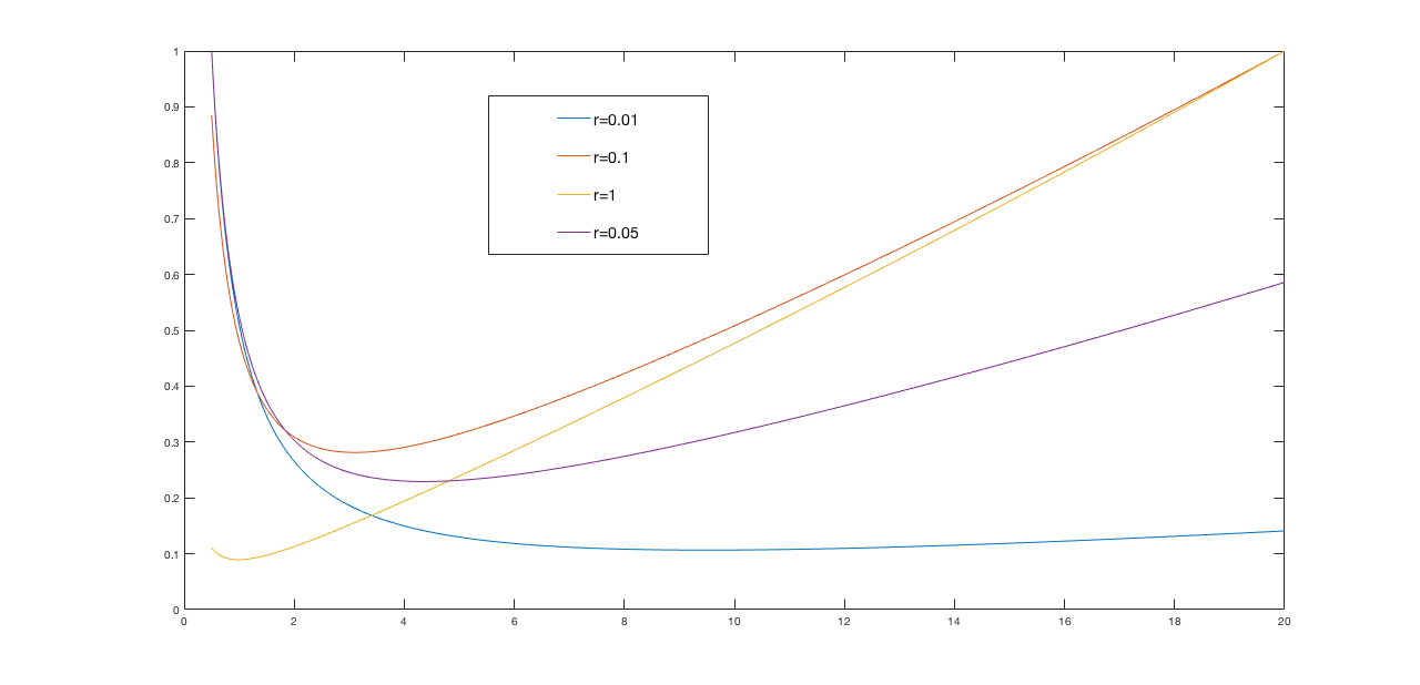
If we set the input weight, r, to almost any non-zero value, optimizing our cost function will lead to far more reasonable gains. For example, below are normalized plots of the cost function

We showed that the LQR cost function for the canonical example,
As we showed above, when picking feedback gains based on minimizing the LQR metric, the initial state is irrelevent, but p is important. That is, we are determining the best k by minimizing p,
For our scalar case, we were able to determine p by summing the series generated by the difference equation (assuming that the system is stable) to show that p is given by
Since we do not know k , and we do not know p , the above equation might not seem that helpful. But it is, as we can differentiate the equation with respect to k,
When we plug the value for k_{opt} in to the equation for p , we get the well-known Ricatti equation for p given the p-minimizing gain. Here, in scalar form, (we let the computer do this algebra),
The invariance of p.
Suppose we were to ask the question, what is the LQR cost function starting from x[1] ? That is, what is
Suppose we let \tilde{n} = n-1 , then
but since the upper limit of the summation is infinity,
The LQR cost to drive x[n] to zero, p x^2[n] , DOES NOT DEPEND ON n! That should not be surprising. If we are presently in San Francisco and want to know how much gas we will need to drive to Los Angeles, it does matter if we started driving yesterday from Seattle, or started driving four days ago from Ottawa.
The history independence of the LQR cost gives us an interesting relationship for p,