Lab 1:
Fast and Spurious
Please Log In for full access to the web site.
Note that this link will take you to an external site (https://shimmer.mit.edu) to authenticate, and then you will be redirected back to this page.
Quick Reference
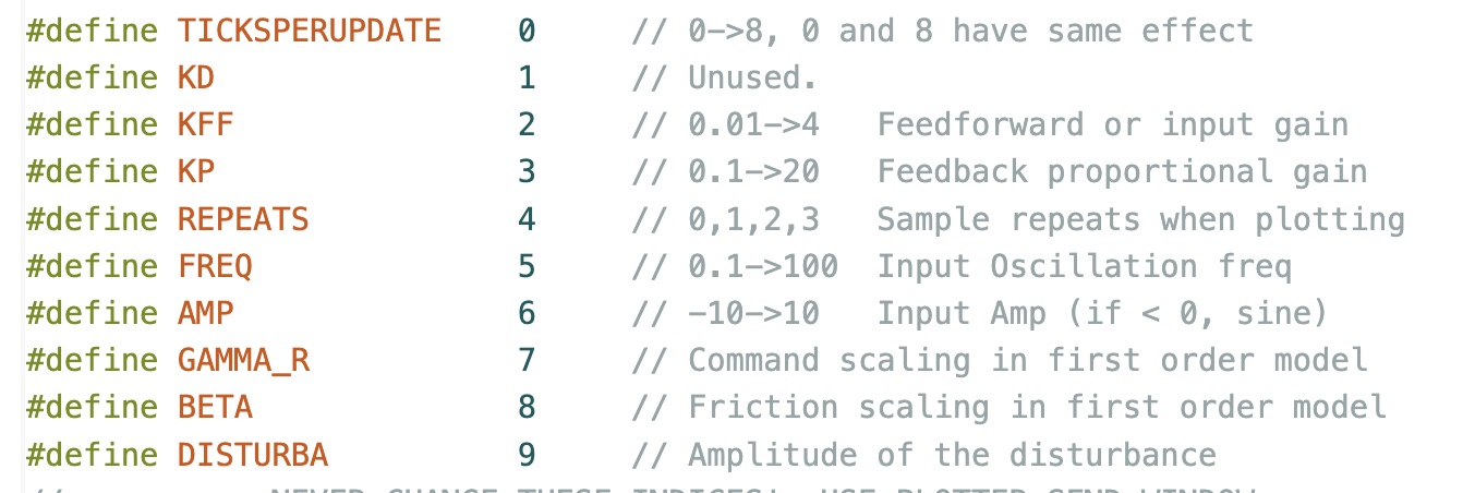
Parameter Indices to use in the serial plotter "Send" window
Links
Task Summary
- THERE IS A TABLE DEFINING SEND INDEXES AT THE TOP OF EVERY LAB!!
- FIND A PARTNER.
- Install Software.
- Build and Test the Speed Control Hardware (checkoff 1).
- Determine the roles of the
ticksperupdate,kff,kp,repeats,freq, andamp, andDisturbA(checkoff 2).
- TBA
Safety First
Please read the EECS Lab Safety instructions.
- We will be building and debugging electrical systems. While everything we do in this subject is low-voltage, you should never modify or even touch a circuit without turning off its power.
- We will be using small but very high speed motors. If our systems go unstable, parts can fly off in any direction. Please wear safety goggles when using the high-speed motors with spinning propellers.
Introduction
The goal of this lab is to control the speed of a motor, while learning about
- Control system modeling,
- Feedback and Stability,
- Sample Rate Effects,
- Steady-state and Dynamic Tracking,
- Insensitivity to Disturbances and uncertainty,
As you will see, the issues associated with control will be obvious and direct, but the issues associated with modeling will be both pervasive and, unfortunately, subtle.
After constructing and testing the speed control system, you will collect data from which to calibrate a first-order difference equation model for the relationship between the Teensy-sketch-generated motor command and the measured motor speed. You will then use this model to make reasonably good predictions about the interactions between sample rates, controller gains, stability, tracking errors, and disturbance insensitivity.
Then, in preparation for the post-lab, you will collect another data set, one specifically designed to expose inaccuracies in the first-order model. As part of the post-lab, you will derive, calibrate, and analyze an improved second-order model, and see if its predictions are better (spoiler alert, sometimes they are).
The take-away about modeling from this lab and post-lab is NOT (we repeat, NOT) that one model is good and the other is bad. As you will see in lab, a first-order model is accurate enough (and simple enough) to answer questions about the interaction between sample rate and stability, or feedback gain and disturbance rejection. But as you will see in the postlab, you'll need a second order model to accurately predict the stability limits on gain, or to predict waveforms near the stability limit.
So, what is the take-away from this lab and postlab about modeling? A good model is usually the simplest model that correctly answers your questions.
Installation and Construction
We use the Arduino IDE 2 software (with modifications and a 6.310 specific library) to communicate with, program, and plot results from our 6.310 controller board (based on the Teensy 4.1 microcontroller). Throughout the term, you will be using this software-board combination, along with lab-specific hardware, to design and experiment with algorithms that control motor speed, rotating arm position, and even magnetic levitation.
Put Together Your Lab Kit. Staff will help you find parts.
Install the Software as described here.
Build and Test the Speed Control Hardware as described in the speed assembly guide here.
After you have carefully followed ALL the steps in the step-by-step assembly guide, demonstrate your working speed control hardware. Demonstrate the operation of your motor by plotting results using mode 0. Describe what is plotted on the horizontal and vertical axes. (Hint: In mode 0, the Teensy samples the optical sensor once every 66.6\museconds.) Describe a method for determining motor speed from this plot. What is the speed indicated by the plot? Change the teensy sketch to mode 1, reupload, and reopen the serial plotter. In mode 1, the speed of the motor is controlled by a feedback system, and the measured speed, desired speed, and motor command are being plotted. The plotted speeds are in thousandths of rotations per second (RPS) minus the nominal speed (set to 15 in the Teensy sketch, or 15,000 thousandths of RPS in the plot). The potentiometer you attached to the controller sets a nominal motor command. What maximum offset from the nominal speed can you achieve by rotating the potentiometer? Use the send window in the serial plotter (DO NOT MODIFY THE SKETCH!) by setting the desired speed to toggle between 14 RPS and 16 RPS every five seconds by first typing Try modifying the feedback gain by setting Try setting a non-zero disturbance by setting the value of
6 1 (followed by return) in the send window, to set the input amplitude to one, and then typing 5 0.1
(followed by return) to set the frequency to 0.1 or the period to 10 seconds. When using the send window, the first number is an integer and is the parameter index (a list of integer-parameter pairs is at the top of every lab) and the second number is the parameter value. Explain what is changing in your plots.Kp using the send window. A feedback term is added to the nominal command when Kp is non-zero, and is proportional to the difference between the desired and measured motor speeds, scaled by K_p. Use the send window to try different values of Kp, be sure to try 1, 0.1, and 0.0. What value of Kp is too large, and why?DisturbA to 0.3 using the send window. Then try increasing the feedback gain, starting from 0.1 and doubling (to 0.2, 0.4, ...). What is the effect of gain on the behavior of the measured motor speed?

Structure of the Control System
The following block diagram illustrates the structure of the speed control system that we will develop.
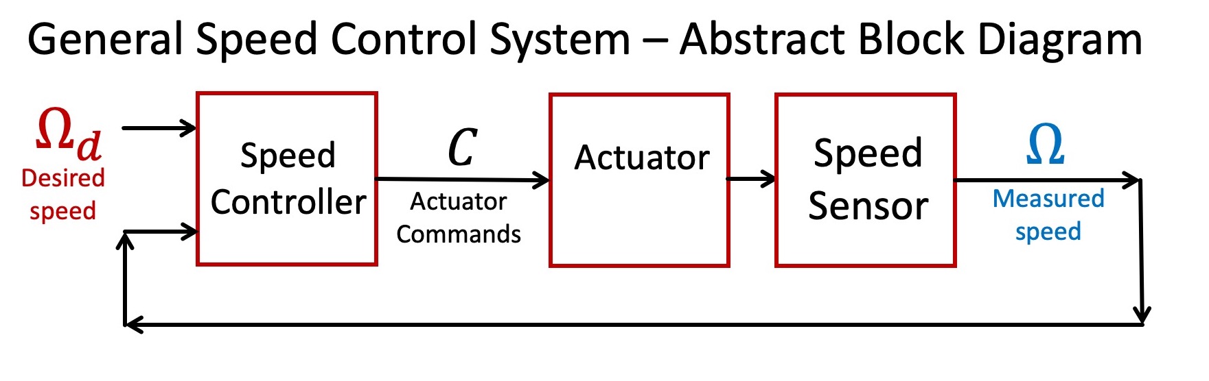
As this diagram suggests, controlling the rotation speed of a spinning object requires three interconnected functions. Foremost of the three is an actuator that can be commanded to either accelerate or decelerate the object. Second, one needs a sensor to verify the object's speed. And thirdly, the focus of much of this class, one must design a controller that can determine effective actuator commands given the desired and measured speeds of the object.
Perturbations from Nominal
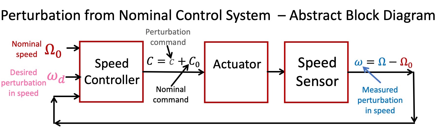
As you may have noticed when testing your speed-controlled motor system, there is a nominal speed of 15 rotations/second (15 RPS), and an associated nominal actuator command. All the other speeds and commands are offsets to these nominal values, so our system is more precisely described by the abstract diagram below. We formulated our speed control problem in terms of perturbations from nominal values partly because it is a natural fit to the common control problem, maintaining constant speed (think automobile cruise control). But more importantly for our purposes, relationships between perturbations are likely to be more linear, and therefore more easily modeled. And good models, as we shall see thoughout the term, are essential precursors to designing good controllers.
Abstracting from Structure
Below is a functional block diagram of our speed control system, based on its physical structures. What should be immediately clear is that the functional block diagram looks nothing like the abstract block diagrams above. For example, is the motor the actuator? Or is it the motor plus the H-Bridge drivers? Also, the combination of the white eight-bladed encoder and the optical sensor does not produce rotation speed, it produces a signal from which the speed can be deduced. So does the combination really form the sensor in our abstract model?
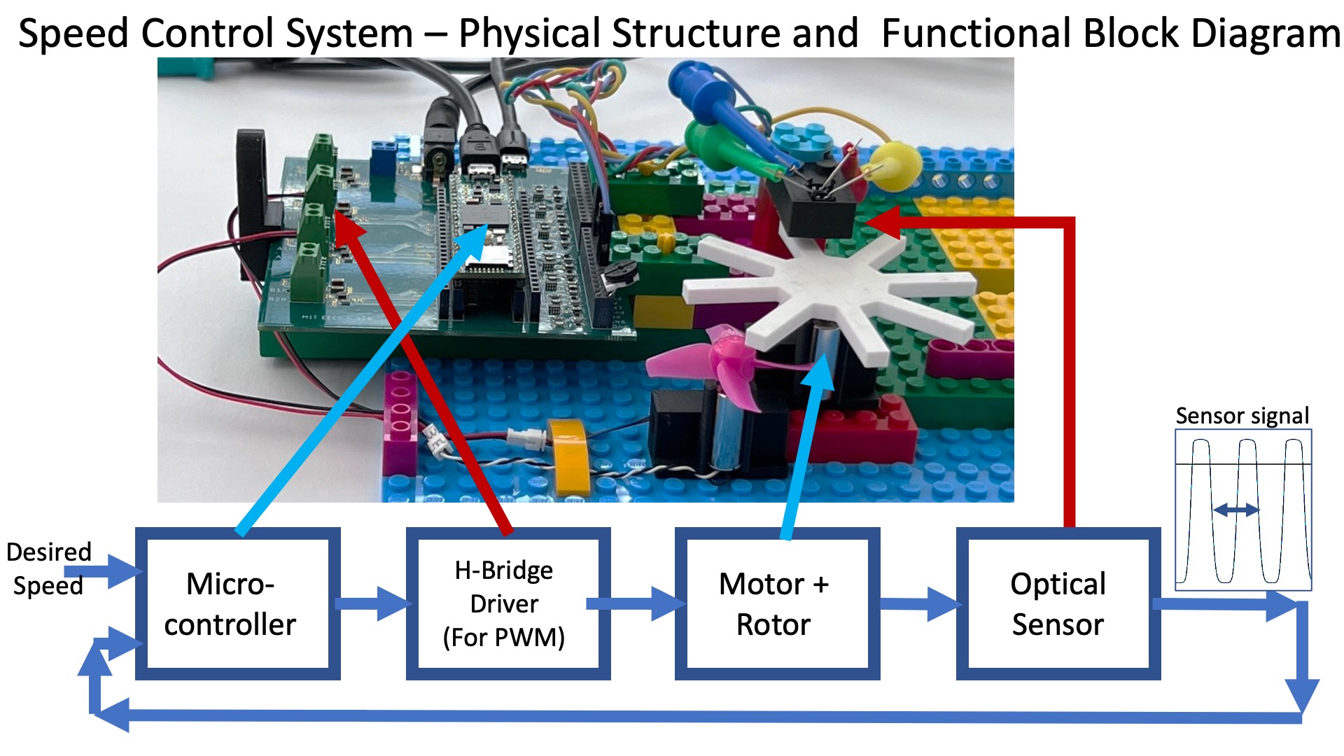
Whether the problem is software or hardware or some combination of the two, finding a good abstract model is often the central challenge in any engineering design. As we noted in the introduction, a good model has enough detail to accurately assess design tradeoffs, yet is simple enough to reveal alternative strategies. But, how does one find a model good enough to answer one's questions, if one needs the model to determine what questions to ask? And how does one find a model that reveals strategies one does not yet know?
Modeling, it is impossible to teach, but fortunately, not impossible to learn.
Connecting Structures and Abstractions
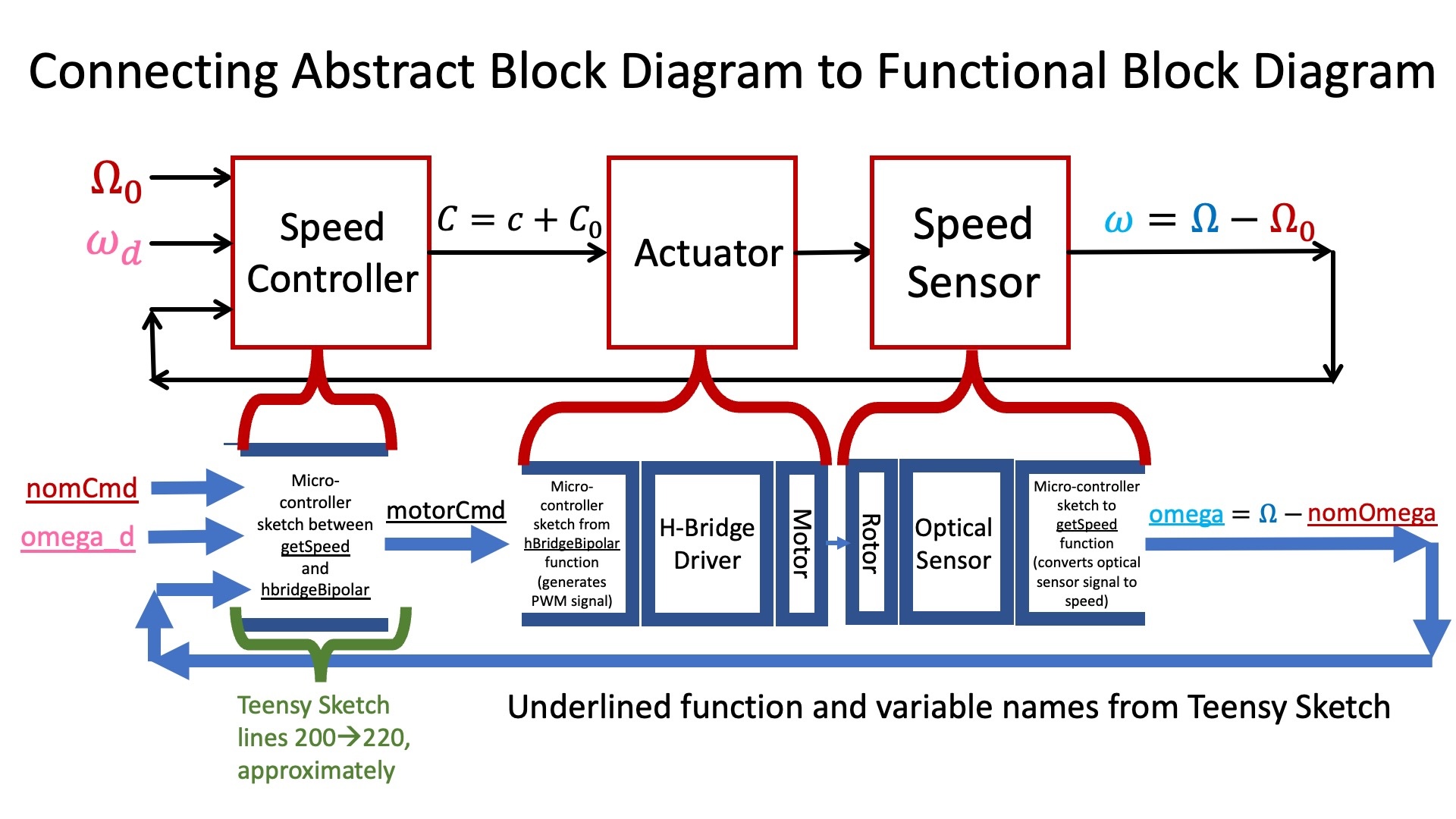
In the case of our speed control system, we can extract an abstract model like the one above provided we ignore the structural boundaries. The speed sensor is a combination of the white eight-bladed encoder, the optical sensor, and the function getSpeed in the Teensy sketch (which converts the time between falling edges in the optical sensor output into speed estimates, see the next section). The actuator in the abstract diagram is a combination of the function hbridgeBipolar in the Teensy sketch (which converts a motor command into a pulse-width-modulated signal), the h-bridge driver, and the motor connected to the white encoder.
We summarize the connection between abstract model and structural implementation in the figure below.
The Controller Block
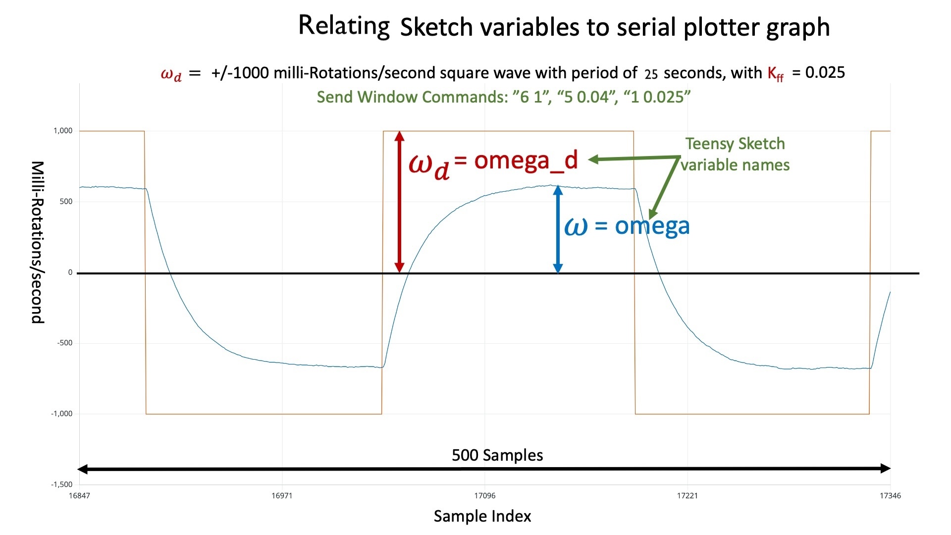
As we can see from the figure in the previous subsection, there is a small part of the Teensy sketch that corresponds to the speed-controller block in the abstract block diagram. The actuator command, motorCmd in the sketch, is computed from the nominal command, nomCmd in the sketch, the desired perturbation in motor speed, omega_d in the sketch, and the measured perturbation in motor speed, omega in the sketch. To make the meaning of omega and omega_d clearer, consider the example plot below. The plot was generated by running the speed control system in control mode (MODE 1), with omega_d set to be a unit amplitude square wave, the controller gain kff set to 0.025, and the square wave frequency set to \frac{1}{25}.
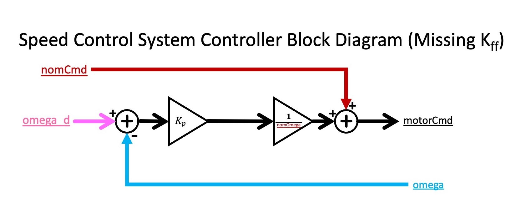
Below we show an incomplete block diagram for the controller, showing how the motor command is computed from the desired and measured motor speeds, as well as the nominal command (which is just added in). The block diagram shows how K_p, the proportional feedback gain, affects the motor command, but does not show the effect of K_{ff}. We will consider adding K_{ff} later in the lab.
Sensing Speed
The optical sensor generates a pulse every time a white encoder blade passes underneath it. More specifically, the blade reflects the infrared light from the led on one side of the sensor to the optotransistor on the other side of the sensor, and when bombarded with infrared light, the optotransistor turns "on". The "on" transistor effectively "pulls-up" the IN5 input on the 6.310 controller board, increasing the voltage from close to zero to nearly three volts. Once the encoder blade passes out from under the sensor, the optotransistor turns "off", the IN5 voltage is pulled back down to zero by a resistor ground (see the schematic in the assembly guide).
The negative change in the voltage on IN5 "interrupts" the microcontroller, which determines the time since the last negative change, and computes the motor speed.
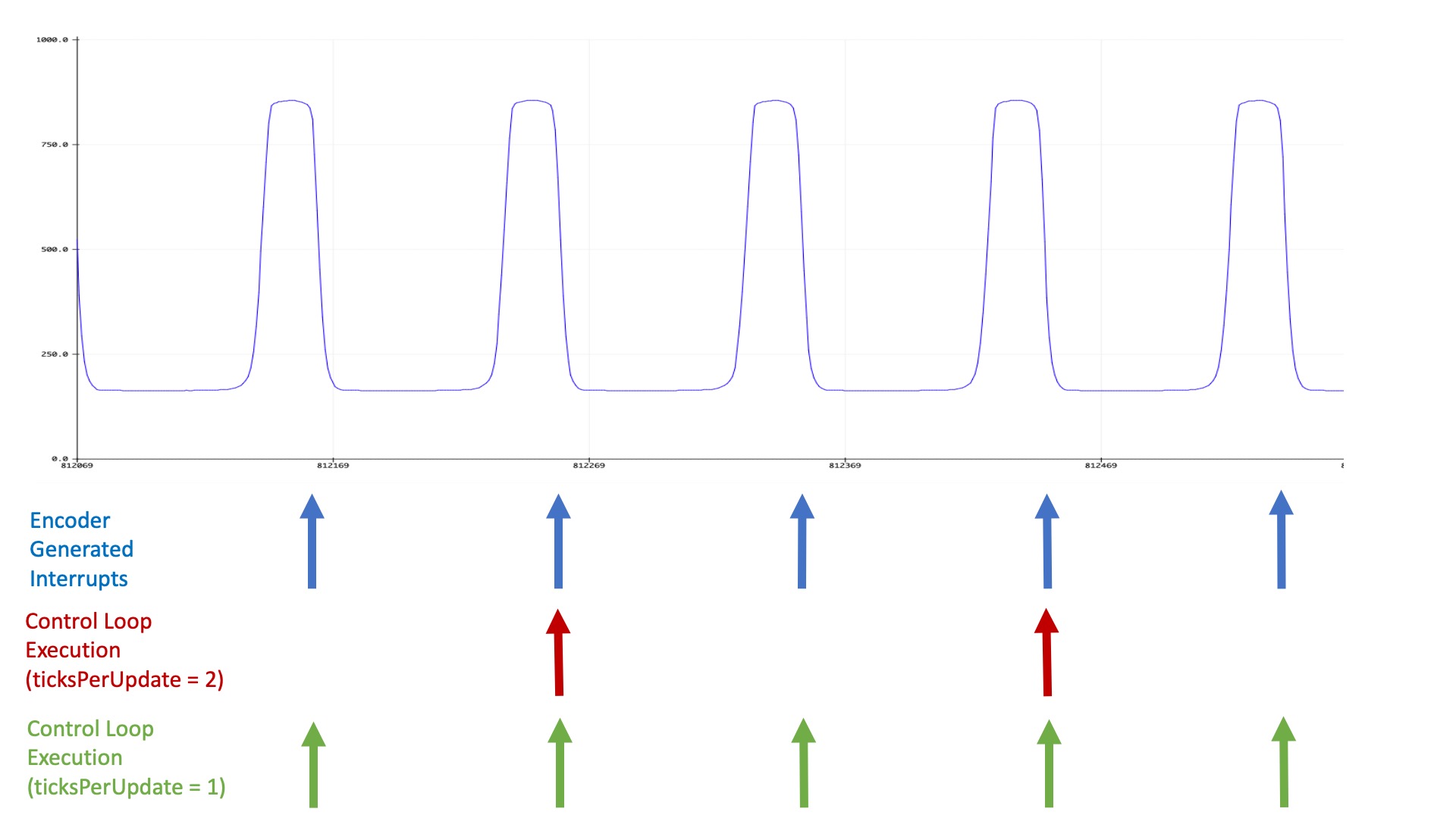
The signal generated by the optical sensor circuit is plotted below (notice the y-axis is normalized, so that 1000 corresponds to three volts), along with a diagram showing when interrupts are triggered on the Teensy, as well as when a control loop (which updates the motor command) executes. As the diagram should make clear, interrupts are generated every time an encoder blade passes under the optical sensor (eight times per rotation for our eight-bladed encoder), but the control loop only runs every m^{th} interrupt, where m is the setting of ticksperupdate (which you change from the serial plotter send window, by typing, e.g. "0 4" to set ticks per update to 4). Note that when ticksperupdate is zero, m is set to the maximum value of 8.
Set the disturbance amplitude to back to zero, and reset the input amplitude to 1 and the oscillation frequency to 0.1 using the send window, and then experiment with modifying For what value of Does changing Remodify sketch to set the disturbance amplitude back to 0.3, what combination of ticksperupdate from 1 to 8.
ticksperupdate is thenoise'' in the
speed measurement largest? Can you explain why the noise level depends on ticksperupdate?ticksperupdate change the effect of K_p? Show plots to demonstrate your result.ticksperupdate and Kp values gives you the best match between desired and measured speed?
STOP HERE FOR THE FIRST WEEK!!!!
Difference Equation Modeling.
As we saw in class, we can construct a difference equation model for our feedback control system and use the model to design a good controller. In general, we approach modeling in three steps:
- Make judicious assumptions to simplify the system,
- Apply a few physical principles to determine a parameterized form of the model and,
- Extract the parameter values from the results of carefully-chosen experiments.
Instantaneous Velocity Assumption
We can derive a first-order difference equation model for the speed control system by assuming that we are measuring the INSTANTANEOUS rotational velocity at the beginning of every control loop execution. We will examine the ramifications of this simplification at the end of this lab (and in postlab).
Model Form
Recall that when first experimenting with the speed control system, we turned a small potentiometer to adjust a nominal motor command, C_0 (nomCmd in the Teensy sketch), to set a nominal motor speed, \Omega_0 (nomOmega in the sketch). We then perturbed the motor command (e.g. by setting non-zero feedback or feed-forward gains) and measured the perturbation in motor speed. In order to model our system more precisely, we will use lower case letters to denote perturbations from nominal,
cmd in the sketch) is the measured perturbation in motor command, \omega[n] (corresponding to omega in the sketch) is the perturbation in measured motor speed, and \omega_d[n] (corresponding to omega_d in the sketch) is the desired perturbation in motor speed.
To start, changes in motor speed can be related to motor acceleration, \alpha, by
As noted above, the sample period is proportional to ticksperupdate, but is also inversely proportional to the motor speed. For example, if we assume the motor is always spinning at exactly 15 rotations per second (RPS) and we set ticksperupdate = 8, then \Delta T = \frac{1}{15} seconds. If we set ticksperupdate = 1, then \Delta T = \frac{1}{120} seconds. However, the motor speed is not exactly 15 RPS, but varies from 14 to 16 RPS, so assuming \Delta T is fixed is an approximation.
Parameter Calibration
One way to generate responses from which to calibrate the linearized model is to use the AMP index in the send window to set the maximum value of omega_d to ten percent of the nominal speed (nominal speed = 15 RPS, so we want to set amp = 1.5 using the send window), then use the KFF index to set K_{ff} so that omega reaches a steady-state that matches omega_d (CORRECT offsets between the desired and measured steady-state by adjusting the POTENTIOMETER!) You will need to set the input frequency low enough so that the motor speed settles between transitions (perhaps 0.05 hertz or ten seconds between transitions, using the send window and the FREQ index). The approach is illustrated in the following figure.
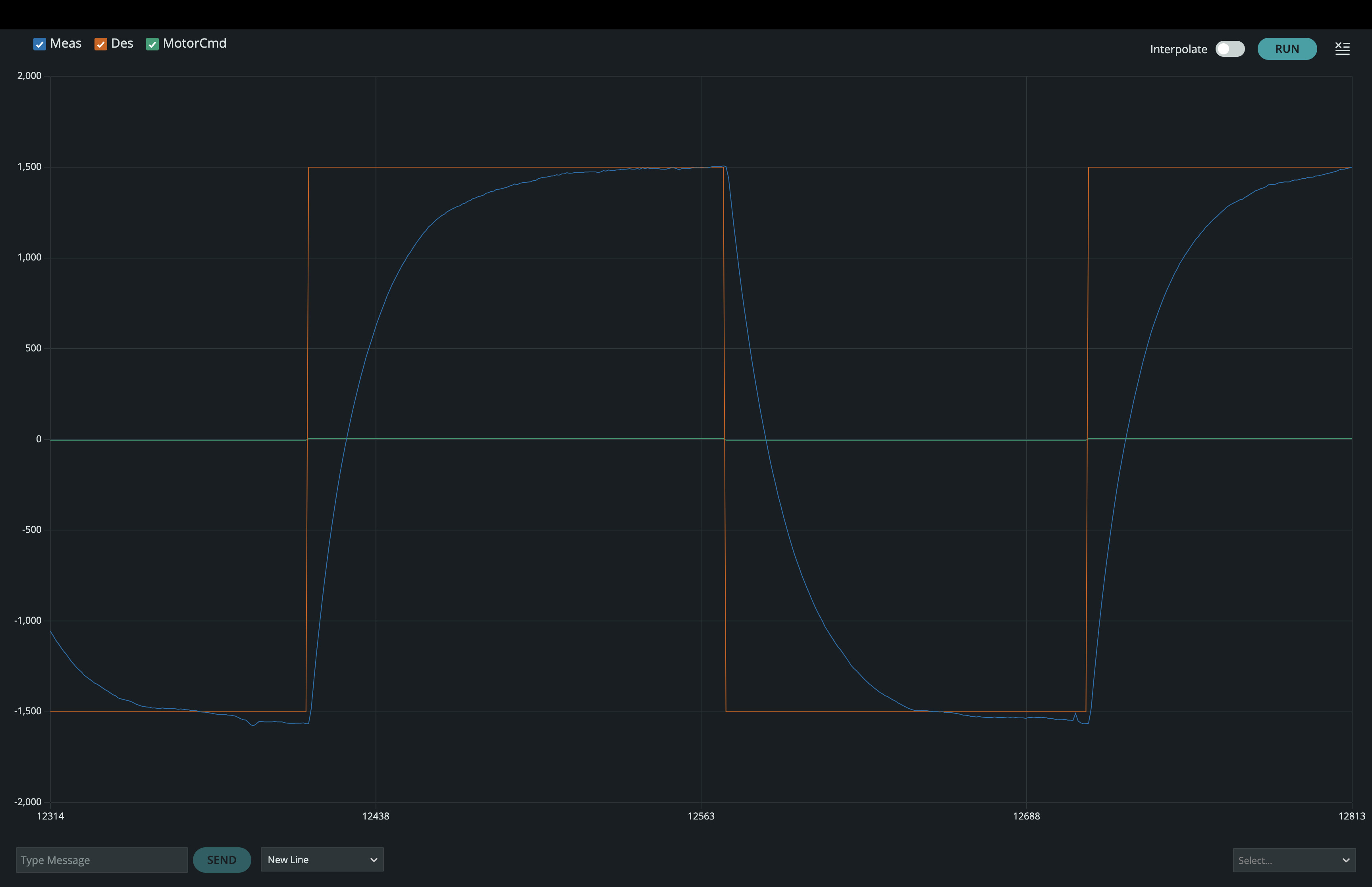
For the above scenario, and in steady-state, \omega[n] = \omega[n-1]= \omega_d[n]. Since
You can derive a second relation involving \beta and \gamma_{r} by examining the dynamic (rather than steady-state) behavior of the perturbed motor speed, \omega[n], in response to the step changes in \omega_d[n]. And the analysis of \omega[n] dynamic behavior will simplify if you exploit the fact that the system is linear, and that both \omega and \omega_d are in steady-state before the step change and eventually in a different steady-state afterwards.
NOTE: You can stop the plot by clicking on the run-stop icon in the plotter, and when stopped, you can move the cursor to any plot to find its x-y values.
Determine the Parameters for Your Motor
There are two coefficients to estimate (\beta and \gamma_{r}), and two types of information in your measured step responses, how fast the measured speed changes and the change in steady-state value.
For this checkoff, determine \beta and \gamma_{r} for your system.
What values did you determine for \beta and \gamma_{r}, and how did you find
them? Please be ready to show screenshots of the data you collected for your calculations (and please remember that you can use the potentiometer to eliminate offsets between measured and desired results!).
Testing Your Model
The generic form for a first-order difference equation (FODE) for \omega[n] is given by
Suppose we use feedback instead of feed-forward in our speed control problem. Then c[n] becomes
Use the above analysis approach to compare model to experiment. For the experiment, use the send window to set the input amplitude to 1, the input frequency to 0.2, and set K_{ff} = 0. Then slowly increasing K_p (starting with K_p=0) and watch the step responses. Determine the value of K_p when your system goes unstable and see if your experiments match your analytic predictions from your calibrated model. Then redo the experiment after using the send window to set the ticksperupdate to 4, then 2 and then 1. For each value of ticksperupdate,
find the maximum value of K_p for which the system is stable, and see if
your experiments match your model's predictions.
ticksperupdate from 8 to 4 and then to 1).ticksperupdate is 8, 4 and 1. Be ready to show step responses on your setup, and to explain what you should you expect, and how do they compare to experiment?
Investigate Disturbances
If we turn on and off the disturbance motor, while also varying the desired motor speed, we are changing two inputs to our system. In the figure below, we plot the behavior of our system as we varied the desired speed and the disturbance (after having set a moderate value for K_p). For the first third of the plotted interval, we varied both the disturbance and the desired speed, for the second third, the desired speed was set to zero and only the disturbance was nonzero, and for the last third, the disturbance was set to zero and only the desired speed was varied. Does the first third of the plot look like the sum of the secondthird of the plot added to the third third? What property of the system would lead you to expect that?
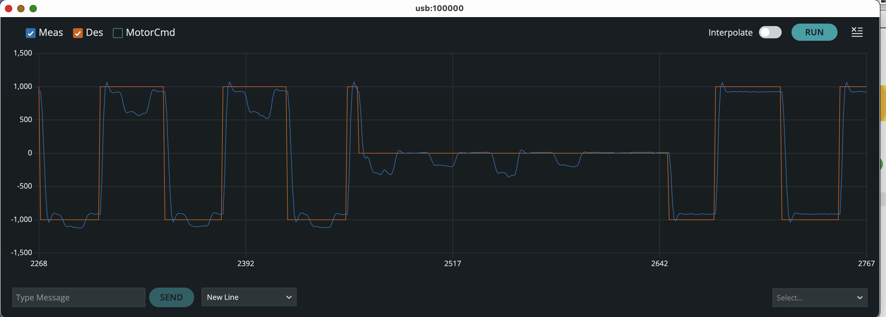
On your system, how does the disturbance rejection vary with increasing K_p?
Try using higher gains by setting ticksperupdate to 4, then 2 and then 1.
What property was our plot above demonstrating? Suppose the disturbance is a constant, and \omega_d[n] = 0 for all n. What does steady-state analysis of your difference equation model indicate about how the the disturbance response scales with K_p? With the input amplitude set to zero, and the disturbance turned on (so the frequency should STILL BE 0.2), determine how the disturbance response varies with increasing K_p (adjust Repeat the above with the input amplitude set to 1. Do the K_p's that minimize disturbance response also produce input responses that settle fastest?
ticksperupdate to four to get higher gains). Does your analysis match experiment?
All Models are Wrong, but Some are Useful.
In creating our model, we assumed that we are measuring motor speed every \Delta T seconds, but are we? We certainly are not measuring motor speed directly. Instead, we are calculating speed indirectly by measuring the time between ticks generated by encoder blades passing under an optical detector. The following figure illustrates our method. When ticksperupdate=8, the control loop runs once after each set of 8 pulses. If we label the current time as t_0 and previous times as t_1, t_2, \cdots, then the sample time \Delta T=t_0-t_8.
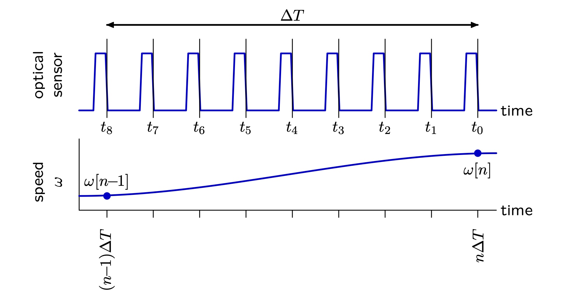
Let \widetilde{\omega} represent our estimate of angular speed based on the experimentally determined times t_i. If ticksperestimate=8, the time for 8 pulses to occur is equal to the time for one turn of the rotor
(since there are 8 blades on the rotor). Therefore the rotational speed is approximately one revolution divided by the time for 8 pulses of light:
In the checkoff below you will investigate the mismatch between the first-order model and the measured results by comparing simulation of the first-order model of the speed controller to your measured data. Recall that the general first order model is
deltaT, Kp, and numerical values for \beta and \gamma_R.
- Download an modified version of today's sketch here.
- Compute
lambdaandgammaon lines 242 and 243 of the Teensy sketch using your numerical values for \beta and \gamma_R and the Teensy variablesdeltaTandKp.Note thatomegaEstis computed on line 244, and is plotted in the serial plotter. For the postlab, you will use the commented out lines just below line 244 to create a second order model foromegaEst. - Upload the corrected sketch to the Teensy, open the serial plotter, set REPEATS=3, ticksperupdate=8, FREQ=0.2, AMP=0.1, and disturbAmp=0. Then find a value for K_p so that the MEASURED rising speed transition oscillates (or
rings ) three of four times before settling. Be prepared to explain the differences between the estimated motor speed and the measured motor speed. In what ways is the measured result inconsistent with the simulated result generated by your first-order difference equation model?
POSTLAB 1.
In this postlab you will modify the Teensy sketch so that it computes an estimate of \omega[n], denoted omegaEst in the Teensy sketch (lines 240->260), using a second-order model. We recomnmend using the following two-step approach to derive the model.
As a first step, assuming
The above second order equation is not exactly what we need if we are asking you to plot model results alongside experimental results. Our experimental setup only measures \widetilde{\omega}[n], so we need a difference equation model for \widetilde{\omega}[n] (which will become omegaEst in the Teensy sketch).
As a second step, please derive the second order model for \widetilde{\omega}[n] in terms of \Delta T, K_p, \beta, \gamma_r, \widetilde{\omega}[n-1], \widetilde{\omega}[n-2], \omega_d[n-1], and \omega_d[n-2].
Implement your model in the Teensy code downloaded for checkoff 6 by modifying Teensy sketch lines 246->249 and uncomment line 250.