The questions below are due on Friday October 02, 2026; 10:00:00 AM.
You are not logged in.
Please Log
In for full access to the web site. Note that this link will take you to
an external site (https://shimmer.mit.edu) to authenticate, and then you will be redirected
back to this page.
You are viewing the PRELIMINARY 6.3100 Fall 2026 web site. Please note that information on this page may change throughout the semester, please check back frequently.
The Matrix Root-Locus and Trajectory Tool is embedded in the Week B section below.
Task Summary
Week A
Build, Calibrate, and Test the Arm Control System (Checkoff 1).
Investigate the behavior of your arm when using only proportional feedback, K_p, and examine the behavior of difference estimates of the derivative as you change the difference interval m (Checkoff 2).
Investigate, experimentally, relationships between proportional and derivative feedback gains and arm performance. Pay particular attention to determining when step responses show the impact of nonlinearity.
Use a combination of proprotional and derivative feedback (by setting non-zero values of K_p and K_d ) to stabilize the arm, and briefly investigate the impact of these gains on disturbance rejection (by dropping a load onto the arm (checkoff 3).
Introduction
In the last lab you modeled and determined control parameters for a motor speed control system, a relatively stationary example, and in this lab you will fly! Well, maybe "fly" is a bit of an exaggeration, though there will be motion. You will build a propeller-thrust-driven rotating arm, and you will control the arm's position by using angle measurements to adjust propeller motor drive. Perhaps a few videos. These videos use a previous term's setup with a propellor on the left and a counter-weight on the right
DO NOT USE A COUNTERWEIGHT FOR YOUR SETUP!!!
Arm Wrestling
In the videos above, we show three propeller arm control systems. In the top video, we show what would happen if we used the same proportional feedback controller we used for speed control. In the bottom left, we show a video of using a PID controller, like the one you will be able to design by the end of this lab. And in the bottom right picture, we show you the kind of controller you will be able to design by the end of the term (after we cover state-space and observers).
The Key Challenge
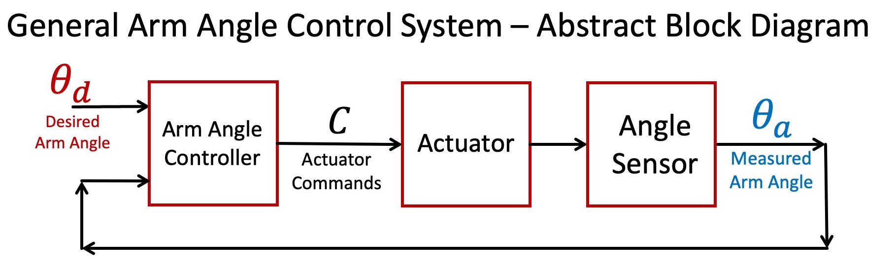
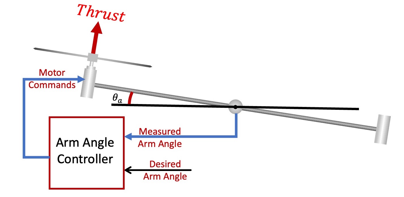
As the abstract block diagram (left panel above) suggests, controlling the rotation angle requires three interconnected functions, an actuator, a sensor and a controller. The angle sensor generates an analog voltage proportional to rotation angle, which is much more direct than the optical encoder sensor used for speed control. But the actuator is more complicated (right panel above). When a motor command is updated by the microcontroller sketch, the voltage across that motor changes, leading to a change in motor speed, which results in a change in propeller thrust, which alters the arm torque, leading to changes in arm angular velocity. The layers of indirection make the control problem challenging, but not uncommonly so, most systems using force-based actuators are similar.
Control Design Approach
Like before, you will model your system and then use the model to help determine a good controller, though for the arm angle control, the modeling and controlling is more complicated. So, you will start with a simple proportional feedback controller, measure the arm behavior, and use those measurements to calibrate a second-order difference equation model of the arm. Then you will use your arm model to determine how the controlled-system's natural frequencies change as a function of proportional(P) and delta(D) (or derivative) feedback gains, and use that insight to design a good PD controller. Success! -ish.
It is possible to find an "okay" PD controller using the second-order arm model, a model accurate enough to predict failure for proportional-only control, but not much more. To achieve better performance, you'll need a more sophisticated controller, and to tune it, you will need a more comprehensive arm model. In particular, you will add an integral (or summation) term to your controller (the "I" in PID), and then tune the three gains (proportional, K_p, derivative, K_d, and integral, K_i) using a model that includes a non-instant relation between changes in motor command and the resulting changes in propeller thrust. And to analyze this complicated controller and model system? For that, you will need to make use of the more sophisticated analysis techniques and computational approaches you've just learned.
Assemble and Test
Please build the propeller-arm control system as described here. Be sure to complete the testing at the end of the assembly guide so that:
the angle sensor axle is oriented correctly,
the measured angle displayed by the serial plotter is zero when the arm is horizontal,
and you've adjusted the nominal motor command so that the associated propeller thrust holds the arm level (that is, horizontal).
Avoid these COMMON PITFALLS!
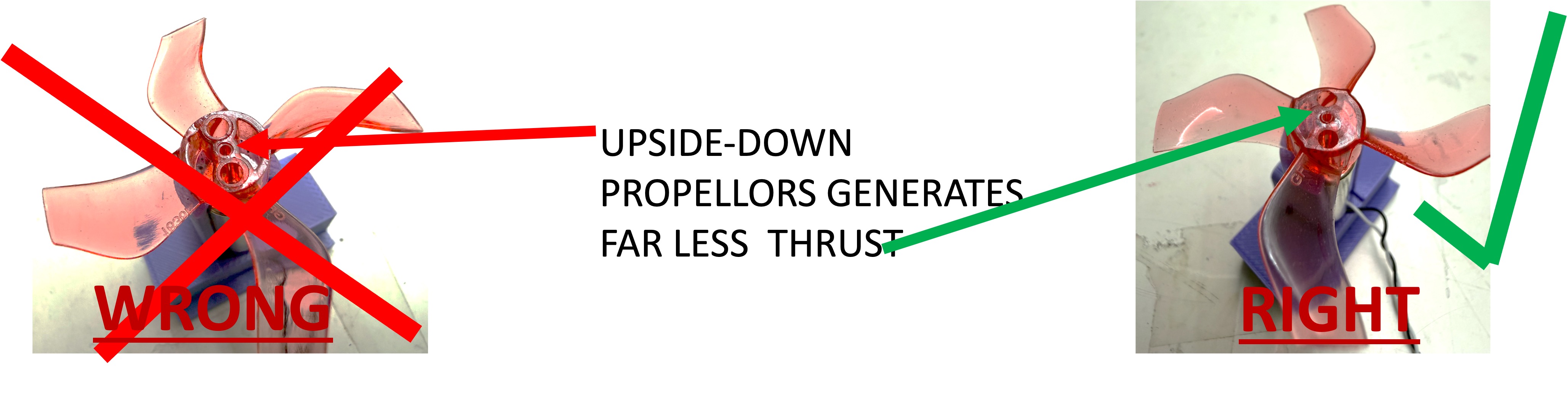
Make sure the propellor is attached to the motor so that the solid surface side of the propellor is pointing up. See the pictures below.
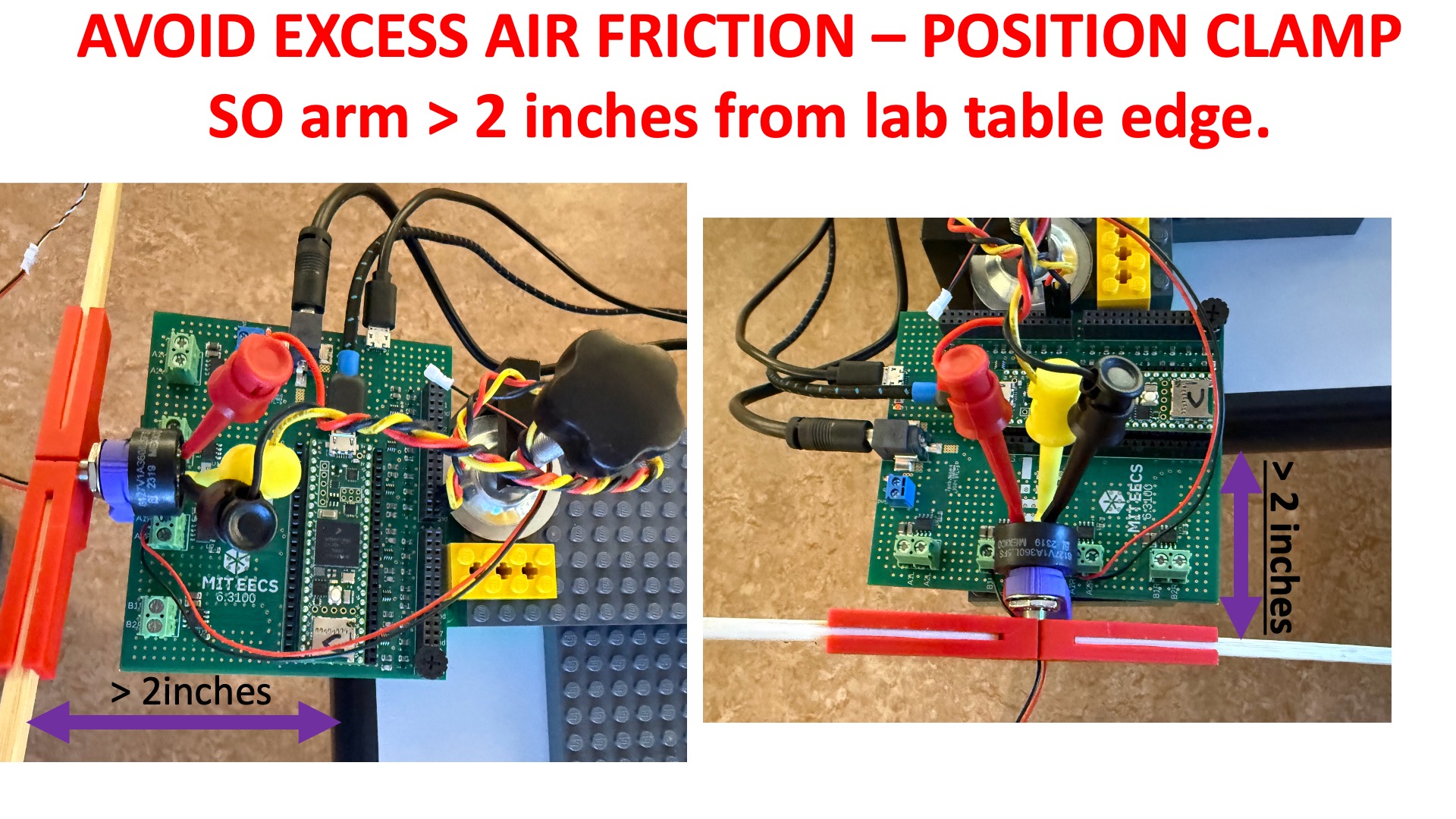
Make sure to clamp your propellor-arm setup to the lab bench so that the arm rotates freely, and is at least two inches from the lab bench.
Checkoff 1:
Demonstrate your calibrated arm.
Use the low proportional gain described in the assembly guide to demonstrate the arm holding itself level. Try blowing on the arm. How well does the arm hold its horizontal position?
Set K_p = 0 and adjust the arm position by turning the potentiometer (the same one you adjusted in lab1) to adjust the nominal motor command (and therefore the propeller thrust). Try to adjust the potentiometer so that the arm is rotated to approximately -0.75 radians (-45 degrees, so BELOW level).
How well does the arm hold this position?
Now adjust the potentiometer so that the arm is approximately +0.75 radians (+45 degrees, so ABOVE level). How well does the arm hold this position?
What fraction of the gravity force on the arm acts to rotate the arm in each case?
What is different about the two arm position? Hint: think about how the gravity force changes when you perturbn the arm angle away from +0.75 radians versus how that force changes when you perturb away from -0.75 radians.
Loading...
Experiment with Proportional Gain
For the second checkoff, we would like you to try some preliminary experiments with proportional feedback, to help you develop an appreciation for the differences between the arm angle and speed control problems.
Determine how the response of the system changes with K_p by using the following procedure:
Use the send window to set K_p (type "3 0.6" for example).
Hold the arm (with your hand) so that the serial plotter shows the arm is about 60 milliradians above horizontal.
Be prepared to stop the plotter -- then let go of the arm!
Stop the plotter, then stop the arm by grabbing the end of the chop stick or by pulling the large power connector.
Repeat with a new K_p
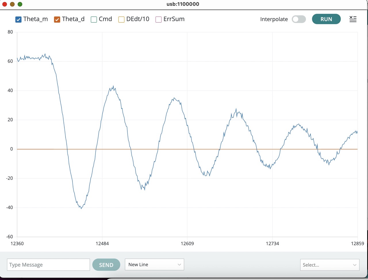
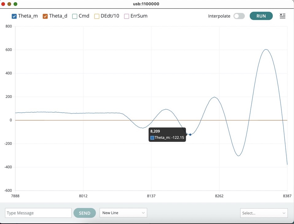
You should be able to find K_p's in the range \frac{1}{4} < K_p < 2 that produce both stable and unstable oscillating behaviors (like the two figures below). Try to find one that is stable (decays to zero like the first figure below), and one that is unstable (like the second figure below). Take screen shots for these two behaviors. You will need them for the checkoff.
Examining Cmd and DEdt/10
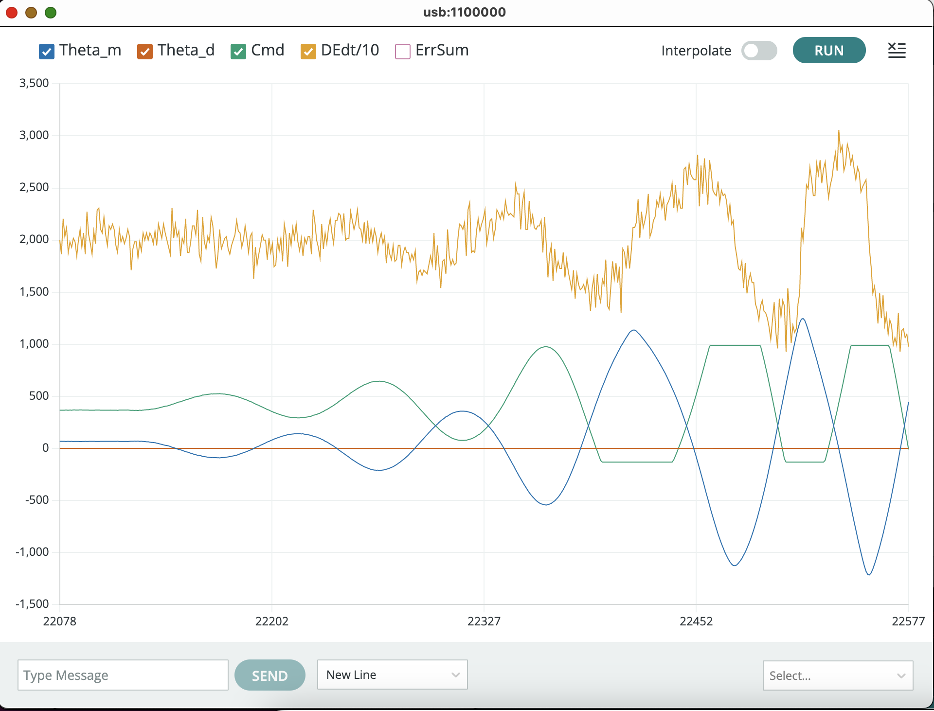
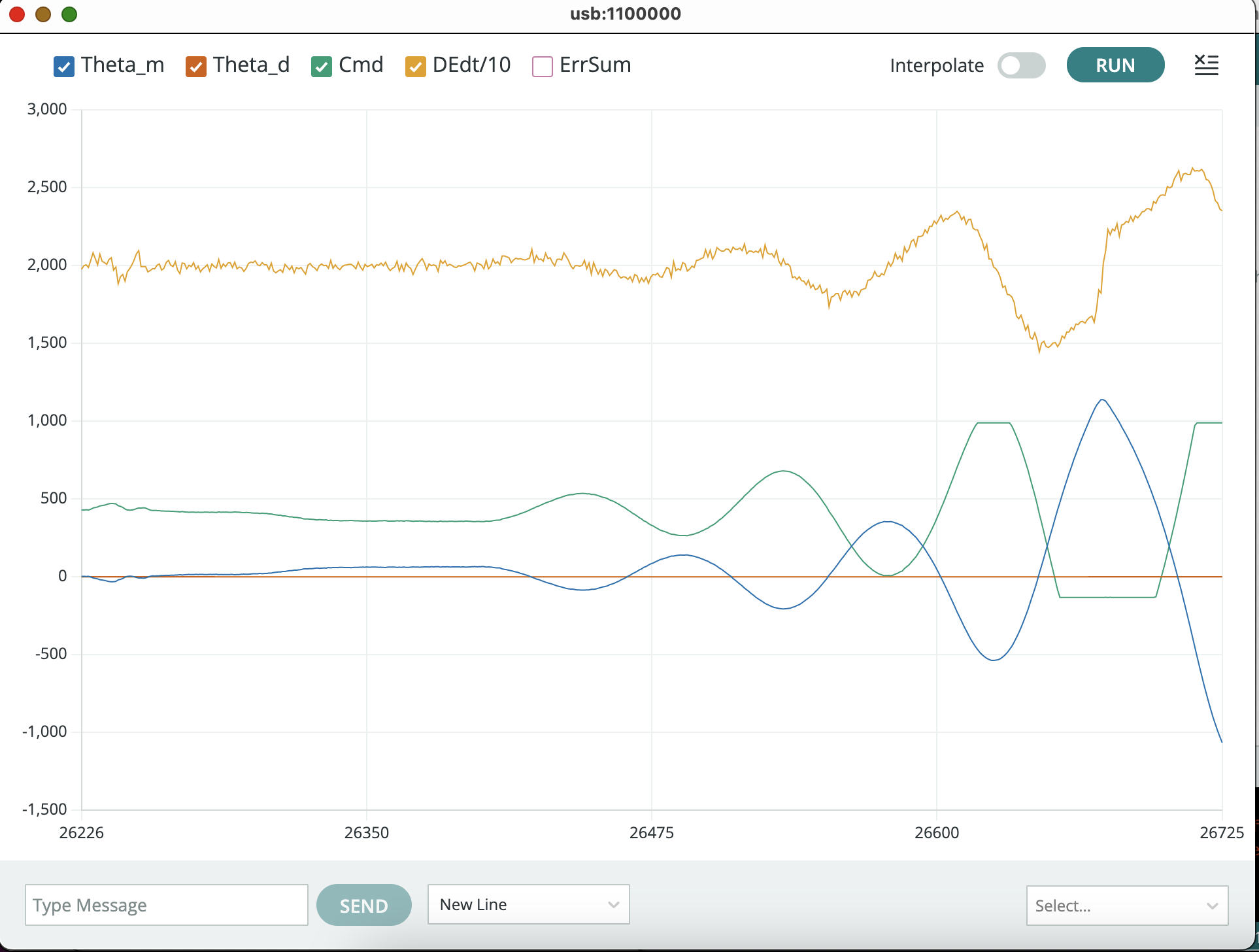
Once you have found a pair of K_p's (one producing decaying, and the other growing, oscillations), turn on the serial plotter plots for the motor command and the derivative of the error, and redo your growing oscillation experiment. You should be able to produce a figure like the one below.
The DEdt plot shows a difference approximation to the time derivative of the arm angle error. The error is defined as the desired minus the measured angle,
e[n] \equiv \theta_d[n] - \theta_a[n],
and the difference approximation to its derivative is given by
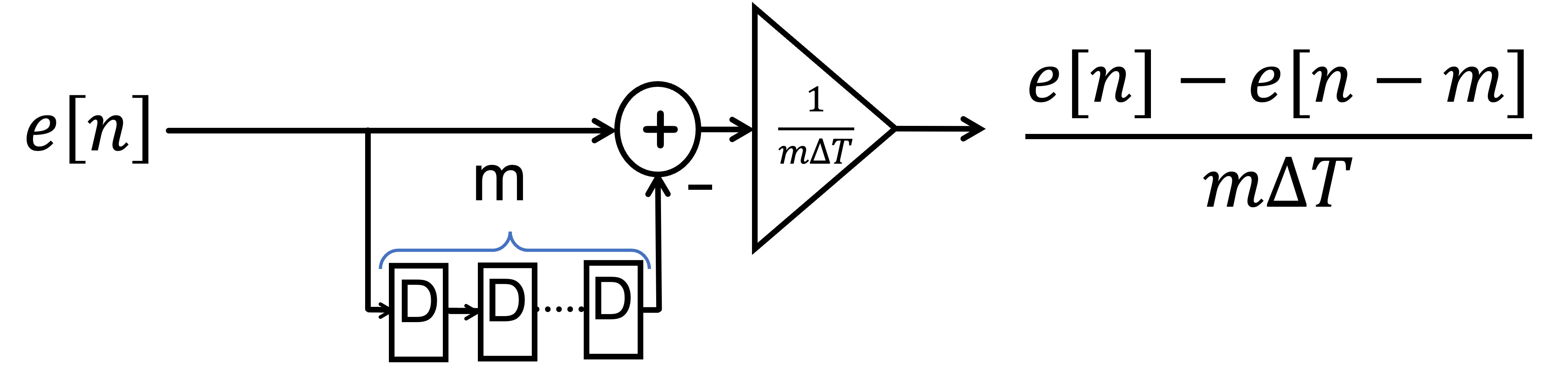
DEdt[n] = \frac{e[n]- e[n-m]}{m\Delta T}
or in block diagram form
where
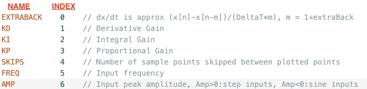
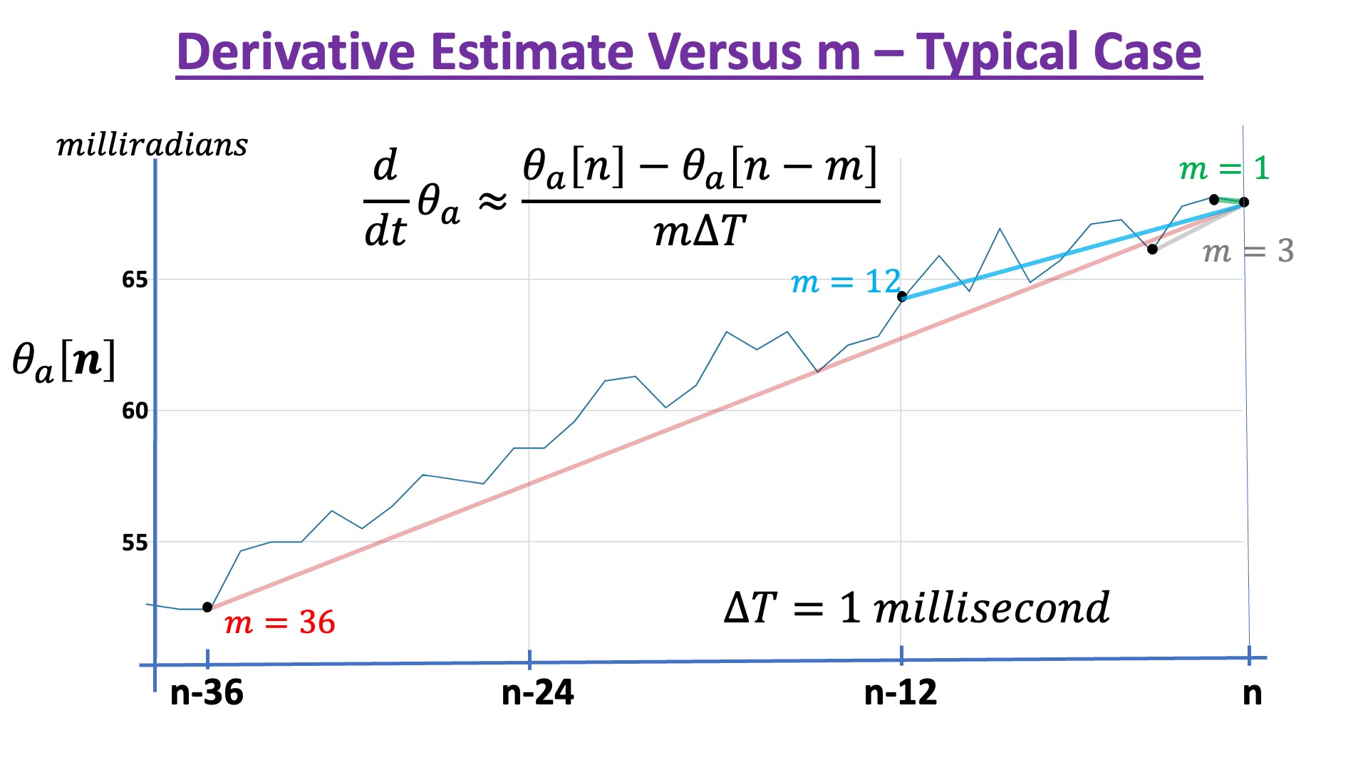
m = 1 + extraBack
indicates how far backward to look for a difference sample . If m is large, the "derivative" is less noisy, but is less "up to date". If m is small, the "derivative" is noisy, but is also more immediate. A typical case is shown in the figure below.
Try increasing m (integers between 1 and 10) using index 0 (EXTRABACK) in the send window. You should be able to set m to produce a figure like the one below.
Checkoff 2:
Show the staff member your screen shots for the largest value of K_p for which your system was stable, that is, the oscillations decayed with a 60 milliradians initial displacement.
Show the staff member your screen shots for the smallest value of K_p for which your system was unstable with a 60 milliradians initial displacement.
What is the relation between the angle, command, and DEdt signals? Do the peaks in these waveforms line up?
How do the waveforms change as m gets bigger? Note that on line 19 in the sketch, #define offsetExtraBack 2 sets an offset of two for EXTRABACK. When you type "0 2" in the send window, you are setting EXTRABACK to four, and therefore setting m=5 . If you want to set m = 1 , type "0 -2" in the send window.
Loading...
Disturbing Observations
At the beginning of this lab you observed evidence of nonlinearity: differences in arm behavior when positioned above horizontal versus below horizontal. And as we saw in lecture this past week, adding derivative feedback, K_d, helped stabilize the path following robot, and increasing proportional feedback, K_p, improved disturbance rejection. So for this last checkoff of part A, we would like you to investigate (experimentally) stability, nonlinearity and disturbance rejection.
Stability and Derivative Feedback
To get a feel for using derivative feedback to stabilize the arm, try the following:
Use the send window to set extraback = 5 (type "0 3" in the send window, to add 3 to offsetExtraBack, which is 2), K_d = 0.2 (type "1 0.2" in the send window) and K_p = 0.5 (type "3 0.5" in the send window). The arm should be level, if not, adjust the potentiometer to level it.
Set the step frequency to 0.1 (type "5 0.1" in send window), and then set the step amplitude to 0.2 (type "6 0.2").
Note the step response, and then try setting K_p = 0.75, then K_p = 1.0, 1.25, 1.5, ... Note how the step response changes with increasing K_p. What is the largest K_p you can use before the system becomes unstable?
Evidence of Nonlinearity
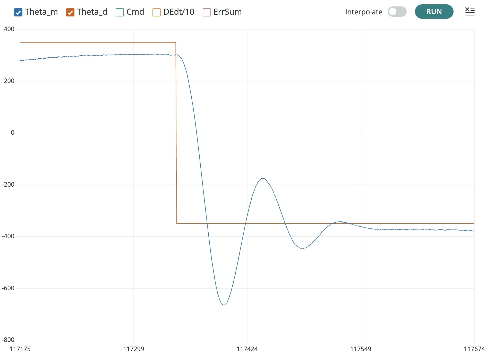
How nonlinearity impacts performance can often be predicted using linear system ideas. Try the following large-step experiment:
Set the step amplitude to 0.35 , K_d=0.1 and K_p=0.6.
Readjust the command offset potentiometer to best match the steady-state-ish values of the desired and measured arm angles.
Decrease K_d until your falling step response oscillates a couple of times before settling down.
Your plot should look something like the plot below (and your K_d should be somewhere between 0.02 and 0.08). What do you observe about the difference between the rising and falling step responses, and can you explain the difference (You will probably need some staff help to answer this one!)?
DIY: Drop It Yourself
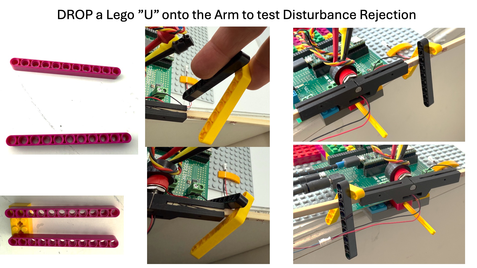
Now lets try disturbing the arm, by dropping a Lego "U" on the arm as shown in the picture below.
TURN OFF THE STEP INPUT, set the input amplitude to zero (type "6 0.0" in the send window)
Set K_d = 0.2, K_p = 0.5, .
Readjust the command offset potentiometer to zero the arm angle.
Try dropping the Lego "U" on your arm and note how the arm angle changes (drop the "U" close to the angle sensor, so it does not have too much leverage, and try to drop it in the same place when you repeat the experiment below).
Try setting K_p = 0.75, redrop the "U", and note how much the arm angle changes. Repeat with K_p = 1.0, 1.25, 1.5.
Checkoff 3:
Please prepared to show and explain your experiments to a staff member.
Stability: What do you observe about the arm step response as you increase K_p?
Nonlinearity: For the large step experiment, what did you observe about the difference between the rising and falling step responses? Can you explain it? (You will probably need some staff help to answer this one!)
Disturbance Rejection: What do you observe about the response to the U-drop disturbance as you increase K_p?
Loading...
STOP HERE FOR WEEK A!!!!
Simple Model, Simple Control
In this section we will derive a second-order difference equation model for propeller arm system based on assuming the motor command and arm torque are related by a single scale factor. We will then determine a numerical value for this scale factor using experimental data.
The Structural and Functional Blocks
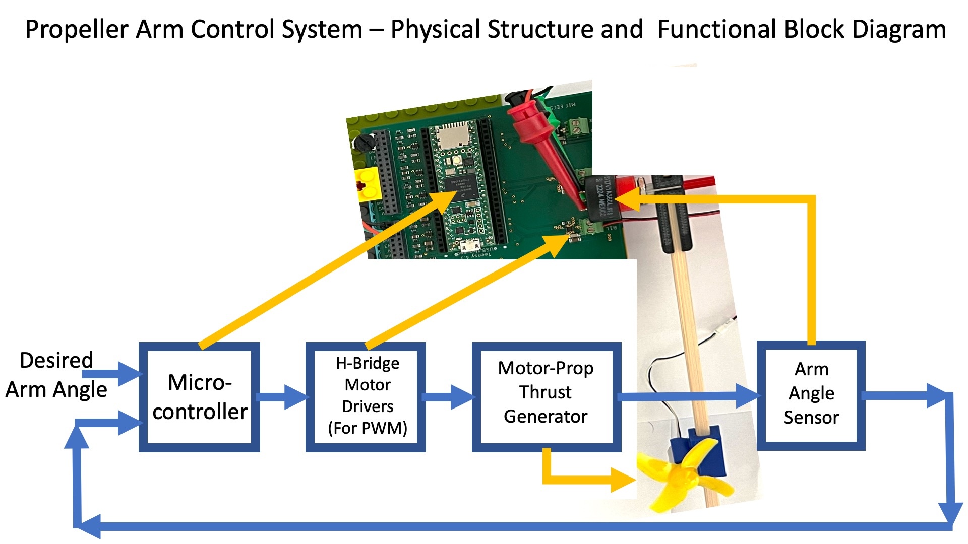
The main structural components of our angle control system are blocked out below.
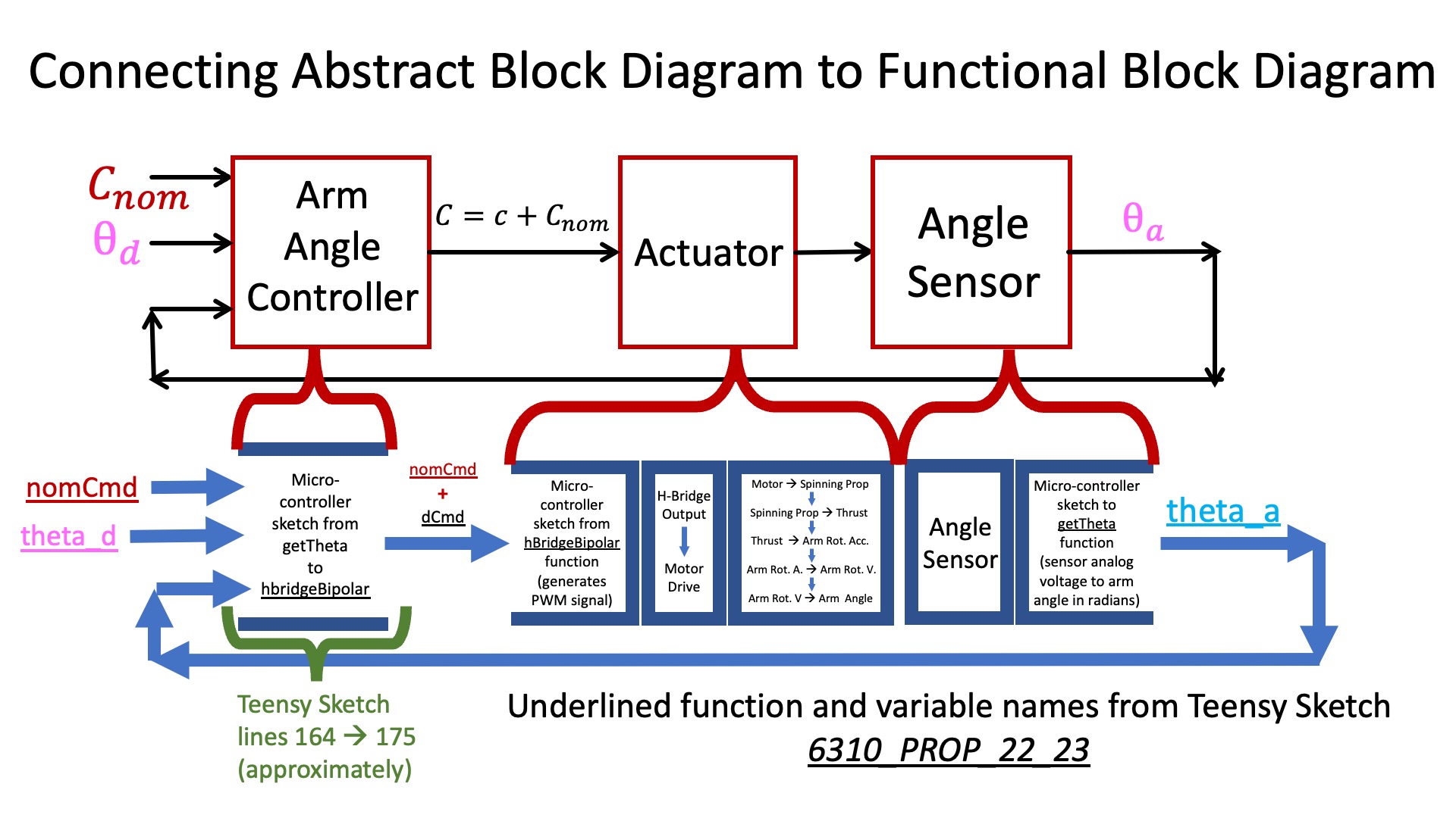
The connection between the structural components and the abstract control functions are detailed in the figure below.
In the above diagram, the command being sent to the actuator (the motor command) is divided into two parts, C = C_{nom} + c. Note that C_{nom} was set to a fixed value during calibration, one that produced enough propeller thrust to exactly cancel gravity when \theta_a = 0 (the horizontal arm case). If we assume that the propeller arm remains nearly horizontal, then we can ignore gravity and the thrust produced by C_{nom}, and focus on relating c ("little c") to \tau_a, the torque responsible for propeller arm angular acceleration.
From Torque to Rotational Velocity to Angle
If \Delta T is small enough, the sampled arm angular velocity can be related to the arm torque by the difference equation
\omega_a[n] \approx \omega_a[n-1] + \Delta T \cdot\frac{\tau_a[n-1]}{I_a},
where I_a is the propeller arm's moment of inertia, and \Delta T is the time between samples in seconds. Similarly, the change in arm angle is approximately
\theta_a[n] \approx \theta_a[n-1] + \Delta T \cdot \omega_a[n-1].
.
We can assemble the above pair of difference equations into a matrix-vector description,
Simple Relation between Motor command and Arm torque
As we noted above, if the c part of the motor command is non-zero, then gravity will not exactly cancel propeller thrust, and the torque produced by the excess thrust,\tau_a will accelerate the arm. The simplest model for the relationship between c[n] and \tau_a is a scale factor, as in
\tau_a[n] = \gamma_{c2t} c[n],
where we have used the subscript c2t to indicate that \gamma_{c2t} relates motor command to arm torque.
Note that we are using a scalar to model a complicated process. The process starts with the microcontroller changing the motor command, which changes the duty-cycle of an H-bridge-buffered PWM signal, which changes the average voltage across a propeller motor, which eventually changes the rotational speed of the motor's thrust-generating propeller, which results in a change in arm torque. Seems like a lot to model with a single number. And in addition, we already know from lab1 that a change in motor command does not instantly change propeller speed, because we modeled that process as part of the first lab.
We know this simple scale factor model will not be perfect, models never are, but some are useful. Let us see if this one is.
As a first step, let us use the model to eliminate \tau_a from our matrix-vector formulation, as in
Note that in the above equation, we have coallesced two parameters into one, by replacing the ratio \frac{\gamma_{ct}}{I_a} with one coefficient, \gamma_a.
Proportional Control
By proportional control, we mean that
c[n] = K_p\left(\theta_d[n]-\theta_a[n]\right)
where c[n] is the perturbation from the gravity-cancelling-at-horizontal nominal motor command, K_p is our proportional gain, \theta_d[n] is our desired arm angle, and \theta_a[n] is our measured arm angle.
If the desired angle is zero (a level arm), \theta_d[n]=0 for all n, then c[n] = K_p\left(-\theta_a[n]\right) and the matrix-vector description becomes
Determine an analytic formula for the complex natural frequencies of the above 2^{nd}-order difference equation model of propeller-arm (the eigenvalues of the the above 2 \times 2 matrix), as a function of \gamma_a and K_p. Use your formula to HAND-DRAW the associated root-locus plot (the eigenvalues versus K_p starting from K_p=0.) in the complex plane. In your drawing, be sure to clearly indicate the unit circle.
Based on your root-locus plot, how will the arm behavior change as you change K_p? Will the arm oscillate faster or slower, will the amplitude of those oscillations grow or decay faster or slower? And what about the behavior of your arm for very small values of K_p? What would you expect based on your root-locus plot, and what do you see experimentally?
As you probably guessed, friction stabilizes the propellor arm when the proportional feedback gain is low, and since friction is not included in our model, the model-experiment inconsistency is not surprising.
Extracting \gamma_a
In Checkoff 2, you found the small values of K_p (proportional gain) for which your arm produced growing oscillations. Oscillations are almost always undesirable when feedback systems are used for control, but are highly desirable when using data to calibrate models. Oscillation frequency is easy to measure precisely, and is particularly informative when that frequency is primarily dependent on a single model parameter. As your root-locus plot above should have made clear, in the simple second-order propeller-arm model, oscillation frequency depends primarily on the product of the model parameter \gamma_a and the proportional feedback gain K_p.
Redo the experiment of checkoff 2 and find the smallest K_p that produces growing oscillations, but this time use a larger starting offset (150 milliradians) and measure the oscillation frequency. Using the larger offset should reduce the K_p needed for growing oscillations, so you should also be able to measure the oscillation frequency for both twice AND half the proportional gain. During each experiment, be sure to pause the serial plotter after two or three periods of the oscillation, when the amplitude is still small and the system is still behaving approximately linearly.
PLEASE NOTE: Keep in mind that \Delta T = 0.001 seconds, and that the plotter plots every tenth sample (so there are one hundred plotted points per second).
By comparing your three measured oscillation periods for three different K_p's to your natural frequency formula, you should be able estimate \gamma_a for your model, and validate your estimate. It may be useful to review the "Polar Form" section of the prelab, here, and take note of the approximation for the magnitude and angle of a complex number z = a + jb when a \approx 1 and |b| << 1. In this case, the magnitude of z,
M = |z| = |a + jb| is approximately 1, and b = M \sin{\phi} \approx \phi.
Enter your measured oscillation period (in seconds) when K_p = K_{p0}:
Loading...
Enter your estimate of \gamma_a:
Loading...
Checkoff 4:
Show your root locus plot and your formula for oscillation frequency version K_p for the second-order model above. For small values of K_p, how does the behavior predicted by your model differ from behavior of your system?
What was the smallest K_p to produce growing oscillations when starting from a 150 milliradian offset? Show plots of the propeller arm under proportional control for that K_p, twice that K_p and half that K_p. What are the three oscillation frequencies for those three cases? Are the frequency ratios consistent with your formula for the oscillation frequency versus K_p.
Try estimating \gamma_a from the three oscillation periods and associated proportional gains. How well do these estimates agree?
Loading...
Friction and Friction-Like Stabilization
Physical analogies can be misleading when first learning about feedback control, but in the case of the propeller arm, we think the spring-damper analogy is quite helpful. So, consider the above proportional control experiments on the arm. After you set a proportional gain, you pull on the arm, then let go and then watch the arm oscillate. That sounds a lot like pulling on a spring, then letting it go, and watching it oscillate. Also, spring forces are typically proportional to displacement from equilibrium, with stiffer springs generating larger forces. Analogously, proportional feedback produces a "force" on the arm that is proportional to the error in angular position, and is scaled by the proportional feedback gain K_p. Increasing K_p increases the force generated per unit displacement, analogous to stiffing a spring.
Pull on a spring, and at least in this reality, its oscillation will not grow in time. That is, springs don't go unstable, but our propeller arm does, a flaw in our analogy. Regardless, the spring's oscillations are "dampened" by friction, so we might expect that friction will stabilize the propeller arm. In fact, we have already seen the stabilizing effect of friction, friction was stabilizing our propeller arm at low proportional feedback gains.
Friction forces are typically proportion to velocity, the time derivative of position, so perhaps it is not so surprising that one can "damp out" the arm's oscillation by adding a feedback term that is proportional to rotational velocity. We can be a little more precise about this, as described below.
Physical Friction
The propeller arm is more stable than predicted by the model analyzed above, and as mentioned before, that is almost certainly because we did not model friction contributions to arm torque. For our propeller arm, the most likely source of arm friction is air resistance which, given the arm's low rotation speeds, scales roughly linearly with arm rotational velocity.
Consider adding a linear friction term to the equation for arm torque,
where \gamma_{c2t} is the coefficient relating motor command to arm torque, and \gamma_{f2t} is a coefficient relating rotational velocity to friction torque.
Using this updated torque formula in the 2x2 matrix representation of our model,
where we again coallesced two parameters into one, by replacing the ratio \frac{\gamma_{f2t}}{I_a} with one coefficient, \gamma_F.
As we will soon see, adding friction to our model has nearly the same effect as using derivative, or velocity, feedback (which you were using last week when you set nonzero values for K_d). This connection can help us develop some intuition about why friction stablizes the arm (because it is like derivative feedback) or conversely, we can reason about the impact of velocity feedback by interpreting it as increased friction.
An aside: If you want to convince yourself about air resistance, try the following experiment on your propeller arm. Set the arm's proportional gain high enough so that when you displace the arm and let go, the arm oscillates with amplitude that decays slowly. Then retry the experiment while holding one of the very large lego plates horizontally, about two inches below the spinning propeller. The air-blocking effect of the nearby plate should increase air resistance, which should visably accelerate oscillation decay.
Velocity AKA Derivative Feedback
Our propeller arm system does not have a sensor for measuring arm angular velocity directly, so the Teensy sketch computes an estimate of the velocity using a difference approximation
where m is the number of "look-back" points mentioned at the very beginning of part 2A of this lab. The Teensy sketch then uses this \tilde{\omega} estimate when calculating feedback commands to the propeller motor.
In the speed control lab, to correctly predict system behavior, it was necessary to incorporate speed measurement details into our difference-equation system model. The slower physical dynamics of the arm (seconds instead of tens of milliseconds) and its faster sampling rate (one millisecond intead of tens of milliseconds) means we can safely ignore those details.
Given the above, the motor command generated by a combination of proportional and derivative feedback is given by
Our finite-difference approach to approximating the arm angular velocity is an example of STATE ESTIMATION, an important topic that we will return to later in term. For now, please note that our justification for the estimation is far from rigorous.
Matrix Root-Locus and Trajectory Tool
In the lab sections that follow, you will investigate improving the stability and steady-state disturbance rejection of your propeller arm controller by adding the discrete-time equivalents of derivative and integral feedback to the proportional feedback you analyzed above. To determine a good weighted combination of proportional, integral and derivative (PID) feedback, that is to determine the gains K_p, K_i, and K_d, will we need a comprehensive model we can use to explore the design space.
We have already seen experimentally that adding derivative feedback stabilizes the arm (when we made K_d nonzero), but there are other consequences. Arm angle derivatives typically change more rapidly than arm angle, so motor commands produced by proportional plus derivative (PD) controllers change more rapidly, rapidly enough to invalidate the above assumption that torque changes instantly with motor command. If we want to accurately predict arm behavior under PD control, we will need a more accurate model of the relationship between motor command and arm torque.
The natural frequencies for the above simplified arm model are the eigenvalues of a 2 \times 2 matrix, and these eigenvalues are easily computed by hand (though the process can become tedious when exploring a design space). Below we will consider using both derivative and integral feedback AND a more accurate non-instant command to torque model. As a result, we will be analyzing larger systems with higher order design spaces. To make the task tenable, we've included a browser-based Matrix Root-Locus and Trajectory Tool (below) that you can use directly on this page.
A Computational Tool
For the rest of this lab, we will focus on using our understanding of natural frequencies to calibrate progressively more complete models of the propeller arm system with PID control. The Matrix Root-Locus and Trajectory Tool embedded below lets you examine eigenvalue (or natural frequency) root-locus plots and zero-input responses directly in your browser — no external software needed. Use it to sweep gains, visualize how the natural frequencies move, and compare simulated ZIR responses to your experimental measurements.
Note that all our natural frequencies are extremely close to one on the unit circle, so the root-locus plot defaults to zoom=True, which crops the view around the interesting region near one, and will drop the natural frequencies near 0. Use zoom=False to see the full unit circle.
Use this tool to analyze a discrete-time state-space system
x[n] = A\,x[n-1]
by entering the system matrix A as a Python nested list.
Matrix entries may be expressions involving any of the five named quantities:
Kp, Kd, Ki, G (for \gamma_a), and B (for \beta).
Matrices from 2×2 up to 5×5 are supported.
Input format: enter the matrix followed (optionally) by comma-separated parameters:
Kp=[lo,hi], Kd=[lo,hi], or Ki=[lo,hi] — sweep ONE gain over a range for the root-locus plot; the others are fixed scalars.
Kp=value, Kd=value, Ki=value — fix a gain at a scalar value (default: Kp=1, Kd=0, Ki=0).
G=value, B=valuedT=value— set the model constants \gamma_a and \beta (default: G=1, B=0, dT=0.001).
x0=[v1,v2,...] — initial condition vector for a ZIR trajectory plot (default: first state = 1, rest = 0). Only used when no gain is swept.
n=[start,end] — sample range for trajectory plots (default: n=[0,40]).
zoom=True or zoom=False — zoom the root-locus panel in around the unit circle (default: zoom=True) (may drop natural frequencies far from one). Use zoom=False to see the full complex plane.
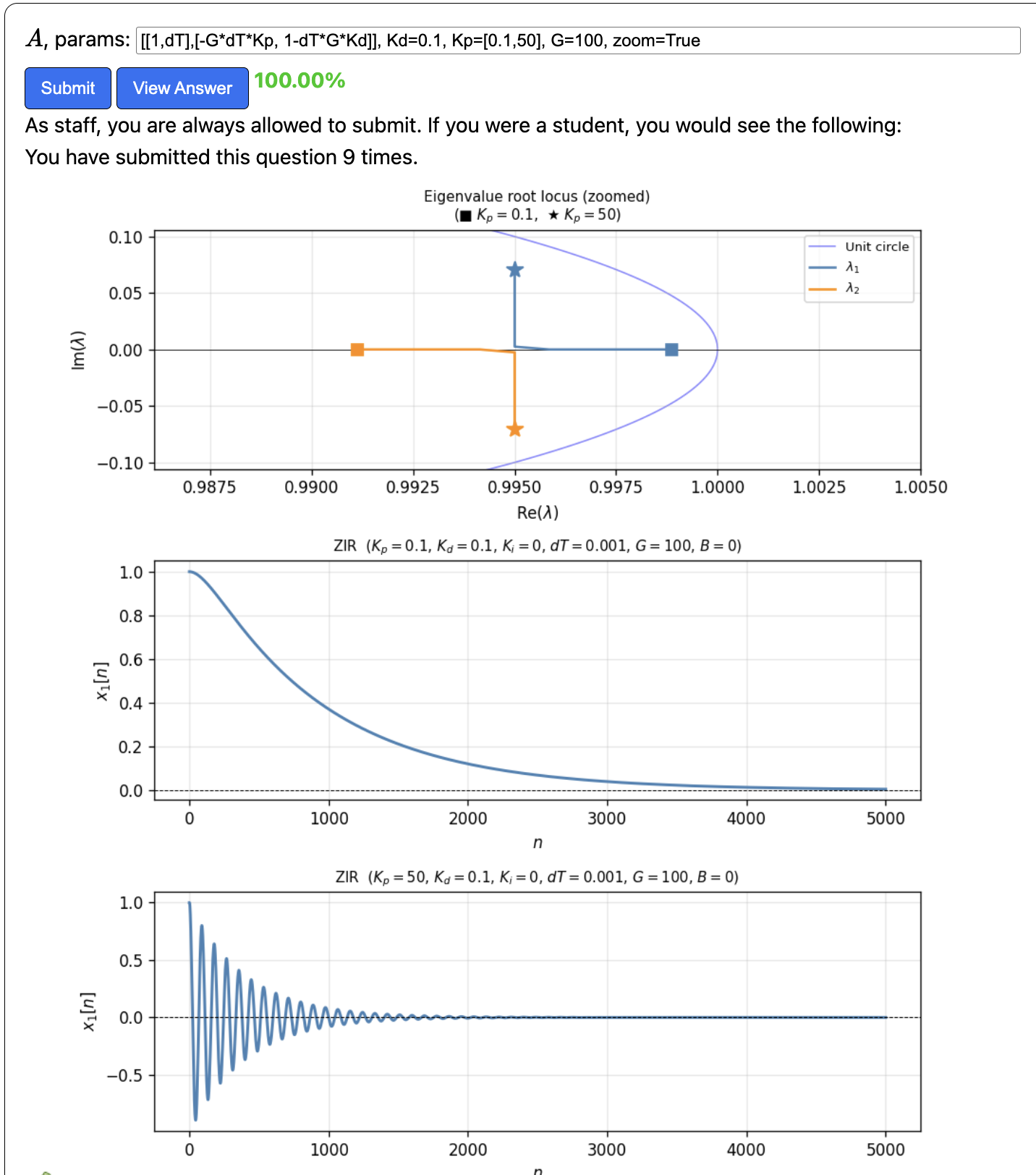
Example — a 2×2 PD arm model sweeping K_p from 0.1 to 50 with K_d=0.1 and \gamma_a=100 specified via G:
Any valid entry earns full credit — this is a design exploration tool.
A, params:
Loading...
You can use the root locus tool to analyze arm controllers with P, PD, or PID feedback, using models parameterized by \gamma_a and \beta (we describe \beta below, for now we set \beta = 0), BUT, the models must be in the form of a parameterized matrix. For example, below we show the above PD example using zoom=True to show the zoomed unit circle.
Please keep in mind that you will need to scale your experimental results when comparing step responses to the root locus tool's ZIR plots (the root locus tool assumes initial arm angle is 1 radian, and all other states are initially zero). Once you have derived the A matrix for your own system, enter it into the root locus tool with your estimated \gamma_a and sweep K_p to reproduce plots like those above.
Motor Command to Arm Torque Model
When the propeller thrust produces arm torque, changes in thrust track changes in propeller speed instantly but nonlinearly, being approximately proportional to the square of the instantaneous propeller speed. Like thrust and propeller speed, changes in motor voltage track changes in motor command instantly, but unlike the propellor-thrust relationship, the voltage-command relationship is linear, with motor voltage being proportional to motor command. One relationship is definitely NOT instantaneous and also not linear, the relationship between changes in propeller speed and changes in motor voltage. Together these observations suggest that a model relating changes in arm torque to changes in motor command will NOT instantious and will be FAR FROM linear, but that is only half right. The motor command to arm torque relationship is suprisingly linear (fortuitous cancellations no doubt), though definitely NOT instantaneous.
Above we used oscillation period measurements versus proportional control gain (K_p) to calibrate \gamma_a, using a model in which we assumed that the relationship between motor command and arm torque was given by
\tau_a[n] \approx \gamma_{ct} c[n],
but as we we noted above, arm torque does not change instantly with motor command.
In the equations for the model of the previous section, arm angular acceleration does not appear explicitly as a variable because we used the instant model and some algebra to eliminate it. But if we want to model the fact that arm angular acceleration does not instantly track motor command, we will need to introduce it as a state variable, and describe its evolution with an associated difference equation. One possible first-order model of arm angular acceleration, \alpha_a, is
where \beta > 0 adjusts the rate of acceleration build-up.
In the above equation, if the motor command is a constant, i.e. c[n] = c[\infty], and \frac{1}{\Delta T} > \beta > 0 , then what is \lim_{n \rightarrow \infty} \alpha_a[n]? And if the the motor command is NOT a constant, but \beta = \frac{1}{\Delta T}, what is the relationship between \alpha_a[n] and c[n].
We can write the vector difference equation for a system that includes the non-instant model
then what are the formulas for A_{3,1}, A_{3,2}, and A_{3,3}. Enter the formulas below using valid python expressions. Also, use B for \beta,dT for \Delta T, (note that dT has a CAPITAL T), G for \gamma_a, Kp for K_p and Kd for K_d.
A31 =
Loading...
A32 =
Loading...
A33 =
Loading...
Implementing and Calibrating the Non-instant model.
Now that you have derived the formulas for A_{3,1} through A_{3,3}, enter the complete 3\times3 non-instant model into the Matrix Root-Locus and Trajectory Tool above, using your own \gamma_a estimate and a starting guess for \beta (try \beta = 5, for example). Try varying \gamma_a and \beta separately in the tool to understand their individual effects:
How does the ZIR change with changing \gamma_a?
How does the ZIR change with changing \beta?
The next step is to find values for \gamma_a and \beta so that the model matches the behavior of you propeller arm. You have two choices: you could try to match up the results from the Matrix Root-Locus and Trajectory Tool (nickname: root locus tool) to the ZIR behavior of your arm OR you could download a new Teensy sketch that automates the ZIR experiment AND simulates your model to allow single screen comparisons.
Calibrating the Model: Approach 1 (NOT RECOMMENDED!)
In the past, we have suggested trying (and taking screenshots of) the following experiments on your propeller arm, and then using the root locus tool above with various values of \gamma_a and \beta until you can match simulation and experiment. To generate a ZIR experimentally, lift one end of the arm (that is, rotate the arm upwards 200 milliradians or so), and then let go.
Set K_d = 0.1 (type "1 0.1" in the send window) and K_p = 1.0
Hold the arm approximate 0.2 radians above horizontal and then let go. Halt the plotter (be quick, so you capture the initial response) and record the result (take a screenshot).
Increase K_p to K_p = 1.5, and then to K_p = 2.0 , and retry your lift-and-let-go arm experiment. Are the natural frequencies and ZIR responses from the root locus tool for these higher values of K_p consistent with your experiments? If not, adjust \beta and PERHAPS slightly adjust \gamma_a and try again.
What makes this strategy such a bad choice? You have be consistent in how you "drop the arm," you have to compare plots from two different programs, and you have to remember how they are individually scaled.
Calibrating the Model: Approach 2 (RECOMMENDED!)
We wrote a new Teensy sketch that implements the experiments in approach 1, and plots measured and simulation results together, just like in postlab 1. You can use the code to determine the values for \gamma_a and \beta for which simulated model matches measurements. You can then use your calibrated model in the Matrix Root-Locus and Trajectory Tool (aka root locus tool) to explore the design space.
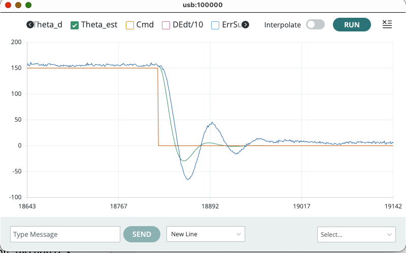
Please download the new sketch here., transfer over the value for the angle offset (line 13 in both sketches), flash the new sketch onto your Teensy, and open the serial plotter. The sketch has been preset to run ZIR responses, so you should see a plot like the one below.
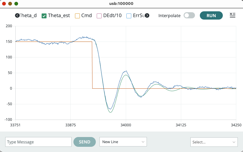
As you can see from the above plot, the model (green) does not match the measurements. If you read through lines 17-50 and lines 170-190 of the new sketch, you should be able to figure how to change the model parameters using the send window until you get a good match like the one below.
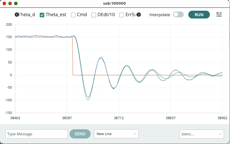
Your model should be predictive, and match when K_p is increased, like in the plot below.
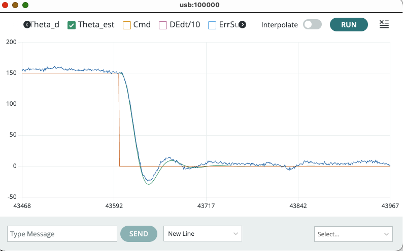
And match when K_d is increased, like the image below.
Enter your estimate of \gamma_a:
Loading...
Enter your estimate of \beta:
Loading...
Checkoff 5:
Describe your estimates of \gamma_a (which should be equal or very close to the value you found in the previous checkoff) and \beta.
What properties of the ZIR are most affected by changes in \gamma_a? What properties are most affected by \beta?
Show us the ZIR responses that you measured and the corresponding responses from the model. How similar are the measured and modeled oscillation frequencies and the rate of oscillation amplitude decay (or growth if your model or experiment is unstable).
Loading...
Better Controls, Models, and Manipulations
PID (Proportional, Integral, Derivative) controllers are ubiquitous in feedback systems, though for discrete-time systems, it would be more accurate to refer to such controllers as PSD (Proportional, Sum, Delta). An ad-hoc approach to designing a PSD controller is to select a proportional feedback gain, K_p, and then increase the gain of the Delta (or derivative) feedback, K_d, until the step response is sufficiently stable. Finally, add Sum (or integral) feedback, with gain K_i, to eliminate any remaining steady-state error.
So if we can easily run experiments, even automate the running of those experiments, what is the value of modeling? With a model we can get far more information that just the result of a single input-output experiment. In particular, we can compute the closed-loop system's natural frequencies as a function of PID controller gains, K_p,K_d, and K_i,, which will tell us how the system will response to a whole of range of inputs and disturbances. In addition, we can even generate plots of how those poles (another name for natural frequencies) move as a function of a parameter, a generalization of the so-called "root-locus" plot. Such plots can tell us what is feasible, like when we used a plot of poles versus proportional gain above to show it was impossible to stabilize the arm with proportional gain alone. Finally, we can use the model to solve a minimax problem with respect to the magnitude of the poles. That is, we could let the computer search through millions of senarios, to find the gains that minimize the closed-loop system's maximum magnitude pole. We would then be sure that resulting closed-loop system would be fast, and that any errors would decrease rapidly. There is much to the story of data and models, some of it with connections to machine learning, and this issue will reemerge many times during the semester.
But we digress. We can add an integral, or more precisely, a sum feedback term to our controller. The advantage of including an integral term is that any persistent error, no matter how small, will cause the sum to grow steadily. When the sum term is large enough, it will cause an adjustment to the motor command, persumably an adjustment that eliminates the small error.
The motor command with the proportional, velocity and sum feedback can be described by the difference equations
where e[n] = \theta_d[n] - \theta_a[n] and sum is the sum ("integral") term. The term involving \omega is not exactly the derivative term associated with a traditional PID controller, but we will return to that issue in the postlab.
When K_i > 0, the error sum becomes a fourth state variable. The third row of the 4\times4A matrix gains one additional entry, A_{3,4}, relating arm acceleration to the error sum state. Derive A_{3,4} and enter it below (use Ki for K_i, G for \gamma_a, B for \beta, dT for \Delta T):
A34 =
Loading...
Implementing and Testing the PID Controller.
In this section you will analyze the new closed-loop system and conduct experiments to understand the model's predictive power. When K_i > 0, the error sum becomes a fourth state variable, extending the A matrix to 4\times4. Once you have derived and checked your formula for A_{3,4} above, enter the full 4\times4 matrix into the root locus tool, using your calibrated \gamma_a and \beta values.
Try the following experiments:
Using the new sketch (6310_PROP_26B), compare the root locus tool's ZIR response (ignore the estimation for now, it does not include the integral term) to your arm's response when K_i > 0.
Once you are satisfied that you have a reasonable match between your arm and the root locus tool's simulation, use the complete model to design the gains of your controller. What are you going to try to minimize? Note: There are practical tradeoffs to make here. The higher the gains, particularly the K_d gain, the more noise in measurement will affect the output. The lower the proportional gain, and the higher the derivative gain, the slower the step response and the greater the error. There is no 'correct' answer, but rather, many answers can be justified. Use the tool and your model!
On line 31 of the new sketch, set the ZIR to 1 (normal operation), set the gains using the other offset parameters, and reflash the Teensy
How is the rejection of transient and steady-state disturbances affected by including the integral (aka sum) term? To see the advantage of using the integral term, try dropping a Lego "U" on the arm.
Checkoff 6:
Demonstrate disturbance rejection as follows.
Find values for Kp and Kd (with Ki=0) so that the measured step response converges within a second. Then increase Ki to decrease the disturbance caused by dropping the LEGO U on the propeller arm. What values of Kp, Kd, Ki work best?
Use the Matrix Root-Locus and Trajectory Tool to find values for K_p and K_d that yield good step responses when K_i = 10.
Try tilting the arm plate and dropping it (DURING THE INTERVIEW!). What do you see?
Compare measured results with and without the integral (sum) term.