Lab 3:A Disturbance in the Force
Please Log In for full access to the web site.
Note that this link will take you to an external site (https://shimmer.mit.edu) to authenticate, and then you will be redirected back to this page.
Quick Reference
NOTE
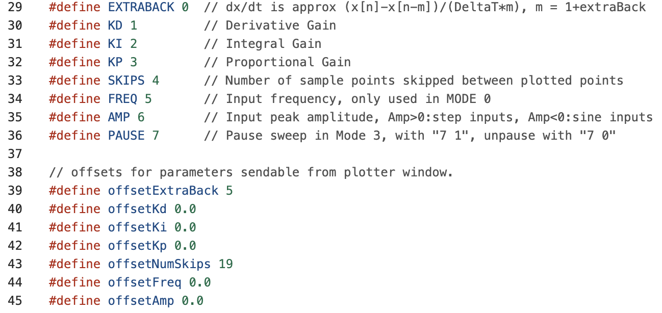
When the sketch is uploaded to the Teensy, it sets K_p, K_d, and K_i to 0.To get non-zero values, you must set them via the serial plotter send window.
Serial Plotter Send Window Indices and Offsets
Links
Task Summary
Week A
- Add a second motor to your arm, download the new sketch, re-calibrate the angle sensor offset, and level the arm (Checkoff 1).
- Set K_i = 4.0, K_p = 0.5, and find the smallest value of K_d for which the system is stable (the step response settles to its steady state after about seven visible oscillations).
- Measure the frequency of the oscillation in the step response, and the magnitude and phase of sinusoidal steady-state responses for several input frequencies (Checkoff 2).
- Set the input to zero (6 0 in send window), then disturb the arm by fanning it, and find the "fanning resonance frequency" that maximizes the disturbance response.
- Consider how the following are related:
- the frequency of the oscillations in the step response,
- the frequency that maximizes the sinusoidal steady-state response,
- and the frequency that maximizes the disturbance response.
- Set K_i=0, K_p = 2, and for this case find a new smallest K_d for which the step response settles after about seven visible oscillations. Turn off the input (6 0), and find the fanning resonance frequency (Checkoff 3).
- Download the IPython file,
ctPropArm.py, to a directory, start ipython in that directory, and at the python prompt type%load ctPropArm.py
Double the fun
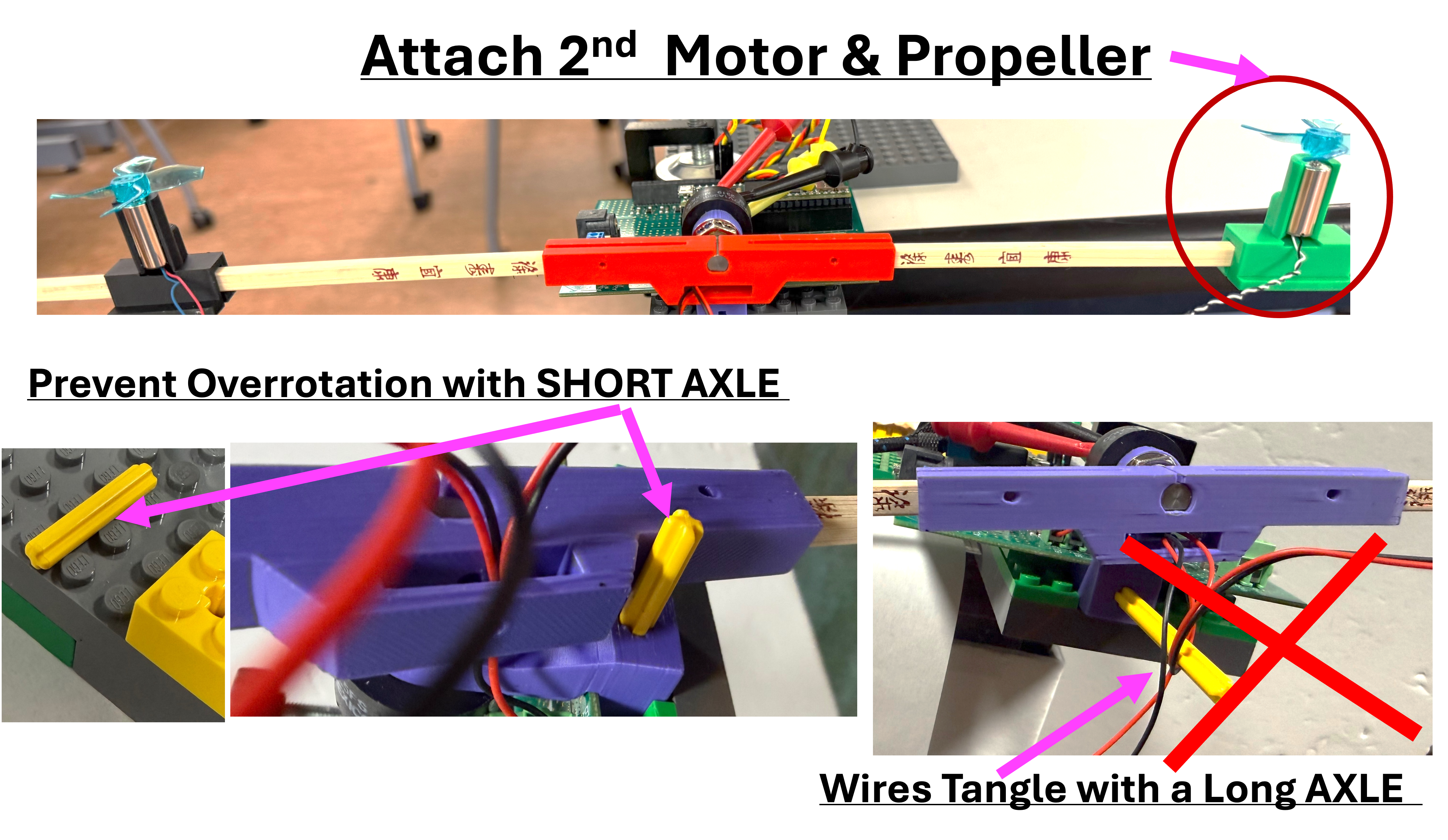
Add a second motor to the right side of the arm, and reclamp the arm to the lab table. As shown in the pictures below:
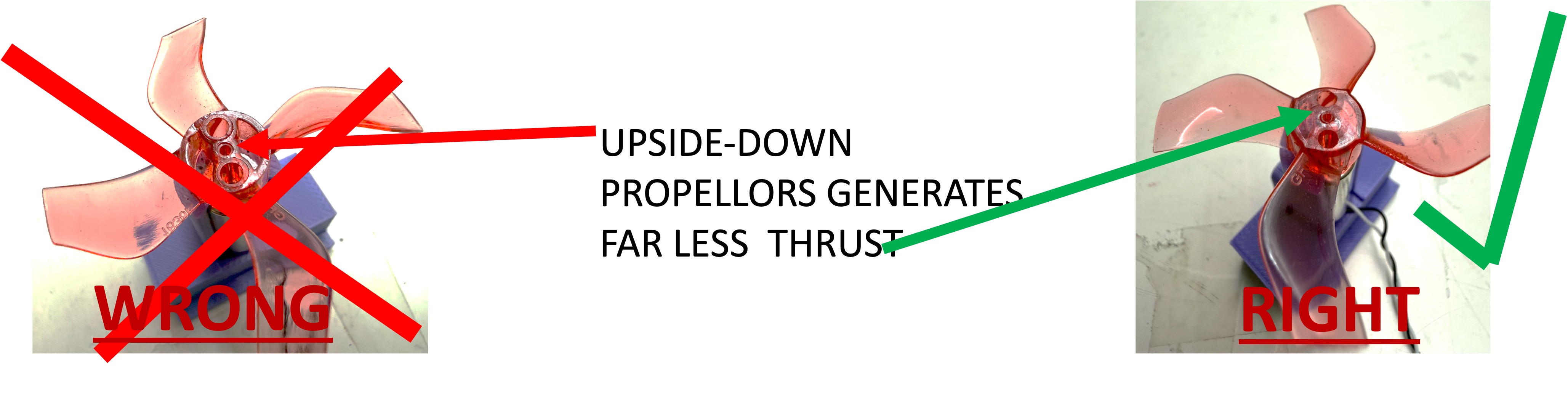
- Be sure that the propellers on BOTH motors are smooth side up!
- Be sure to use a SHORT axle to prevent over-rotation, long axles can get tangled in the wires.
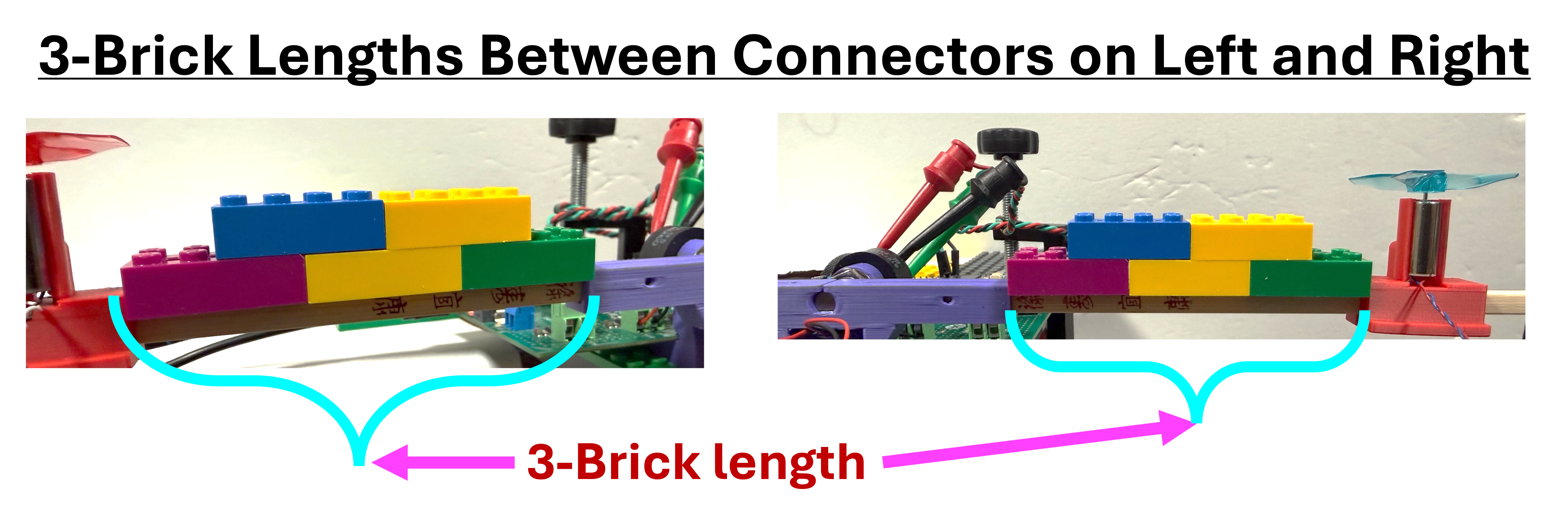
- Be sure to separate the propeller connector from arm connector by three brick lengths on both the left and right sides.
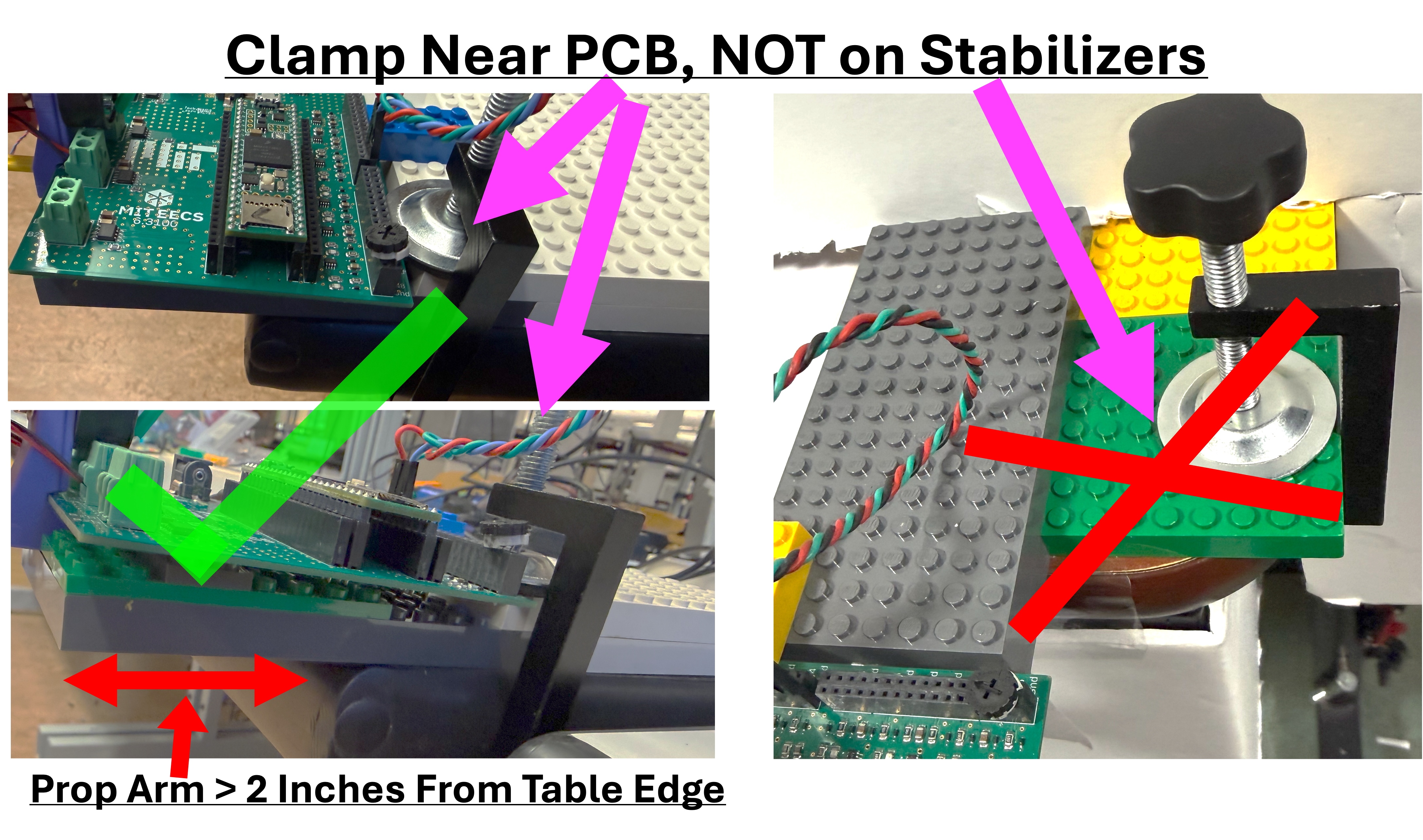
- Securely clamp your arm to the side of the lab table. The clamp should be close to the PCB and the propeller arm should be at least two inches away from the lab table (to minimize air resistance).
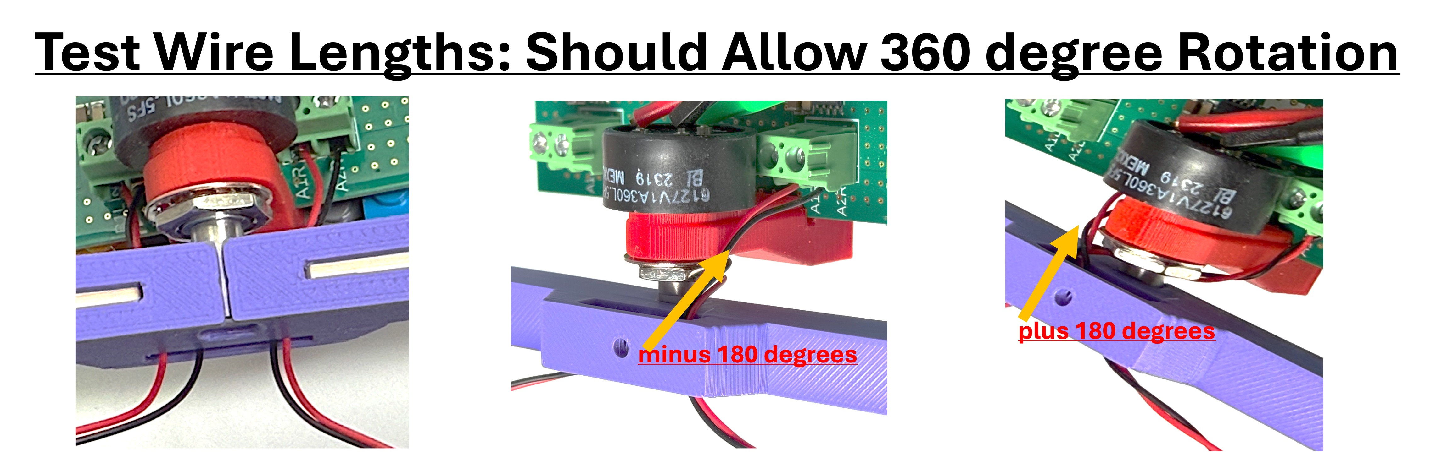
- Check that the wiring allows the arm to rotate from -180 degrees to +180 degrees, or from -\pi to \pi radians (you will need to remove the axle to check this, be sure to reattach it afterwards).
Power up the Propeller Arm
Connect both power supplies (the 5V USB power supply AND the 5V 10 amp power supply) to the controller board and connect your laptop to the Teensy. Download the sketch linked at the top of this page, upload it to the Teensy, and start the serial plotter. Note that the offsets for K_p, K_d, and K_i are all zero. Below you will change these gain values to get enough feedback for the arm to level itself.
Hold the arm level and ensure the plotter shows a zero angle. If not, adjust the AngleOffset in the Teensy sketch (you may be able to use the same AngleOffset from the week 2 sketch). Once the sensor is calibrated, stop holding the arm, and try to level the arm by adjusting the black potentiometer (in the upper right hand corner of the board). The potentiometer can be used to adjust the relative thrust of the right and left propellers, so that the arm holds itself level (set K_p = 0.1 first, otherwise the arm will just drift).
Tip: If your motors are not turning, here are some troubleshooting steps:
- Is the high-current power supply (round connector) plugged in?
- Did you download the sketch for Lab 3 and upload it to your Teensy?
- Check the connection between each motor and its extension wires. It is very easy to bend the pins in the extension wire connector, THIS IS THE MOST COMMON ISSUE!!! Get new extension wires!
- Check the connection of the extension leads to the screw terminals on the circuit board. There should be about 3mm of bare silver wire for the connector to grab, and it should be invisible outside the screw terminal. If uninsulated silver wire is visible outside the screw terminal, that wire could "short" and damage the board.
- Use a multimeter (there are about a dozen of them distributed around the lab, ask for help) to check the potential difference across the two terminals at the controller board. Touch the multimeter voltage probes to the screws and check if there is a non-zero voltage; if not, feel free to ask staff for help.
Tip: Make sure that both propellers are blowing air downwards. If they are not, there are two ways to fix this: swapping wires or editing the code. EDIT THE CODE, it is much easier. Find lines 278 and 280 and swap the order of B1L and B2L or A2R and A1R, depending on which motor needs to be changed; note that these ports are labeled on the PCB.
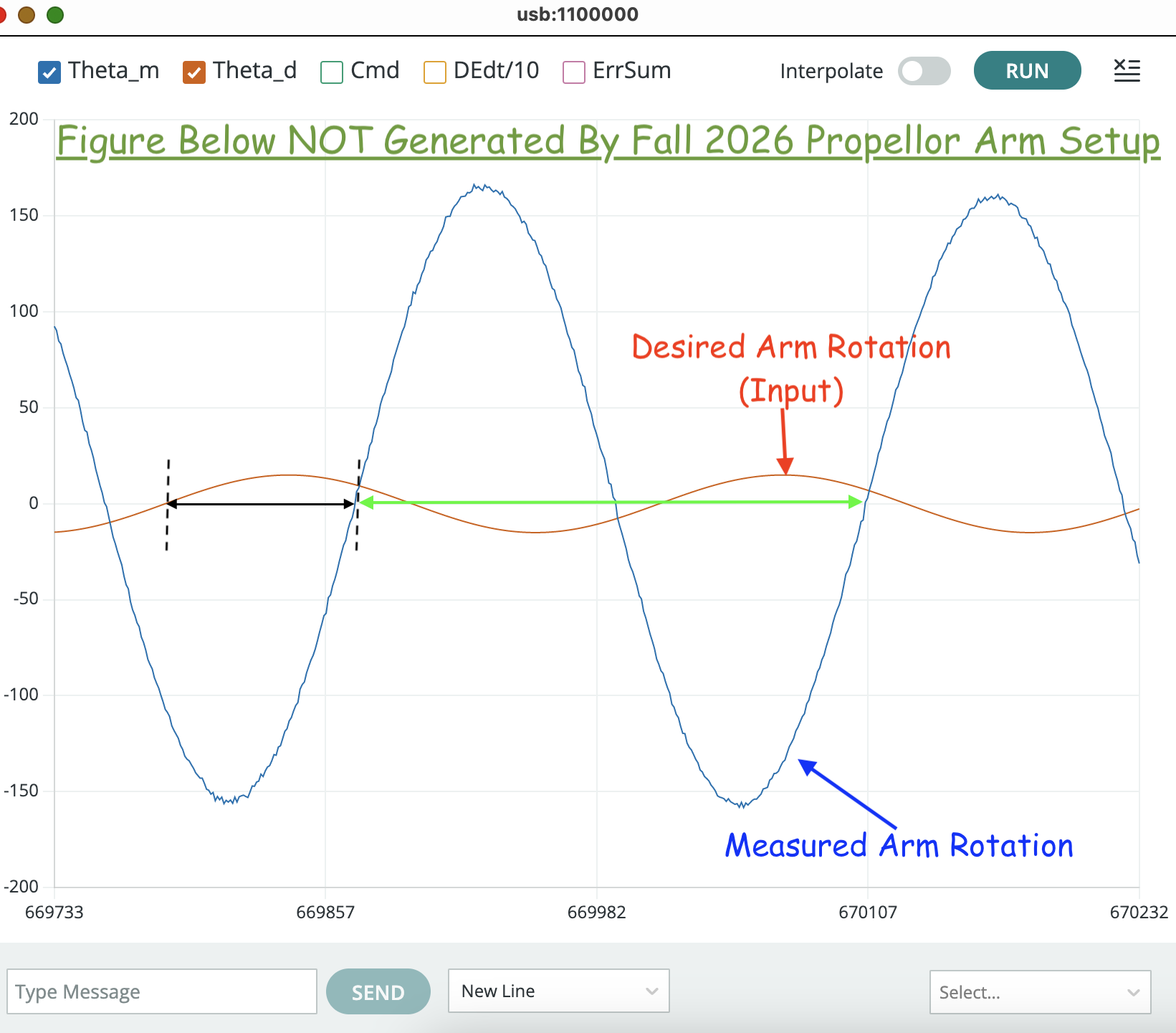
The figure below shows serial plotter output from running this lab's sketch on a propeller arm (from a prior term of 6.310!!!) with a sinusoidal input (in red) and the resulting measured angle (in blue). Notice the two intervals measured on the plot, one denoted with a black double arrow and the other with a green double arrow. How does the ratio of those two intervals relate to the phase difference between the two plots?

Steps, Sinusoids, and Disturbances
Step response
Set K_p=0.5; K_d=0.3; K_i=4.0 and then type "6 0.1" and "5 0.05" to generate an input that is high for 10 seconds, then low for 10 seconds, and then repeats (note that the plot window is 10 seconds wide, and the plot points are 20 milliseconds apart). Then try a few different values for K_d. You should be able to find a K_d between 0.1 and 0.3 that produces a QUALITATIVELY similar step response (its step response should oscillates as much) to the step response shown in the following video (an earlier version of the propeller arm was used in this video, do not try to compare numerical values!!). Notice that in the video, the step response visibly oscillates about seven times before settling; the step response of your arm with your selected K_d should oscillate similarly (seven visible oscillations).
Measure Frequency Response
In theory, measuring the frequency response of a STABLE linear system is easy:
- Pick a frequency and apply a sinusoid of that frequency to your system's input.
- Wait for the system's natural responses to die out (they must die out eventually, since the system is stable). What remains will be sinusoidal at the same frequency as the input.
- Compare the input sinusoid to the output sinusoid and compute the amplitude ratio and the phase difference.
We can measure the frequency response for our two-propeller arm system using the above approach as long as we are careful about the three issues described below.
Monitor Motor Commands
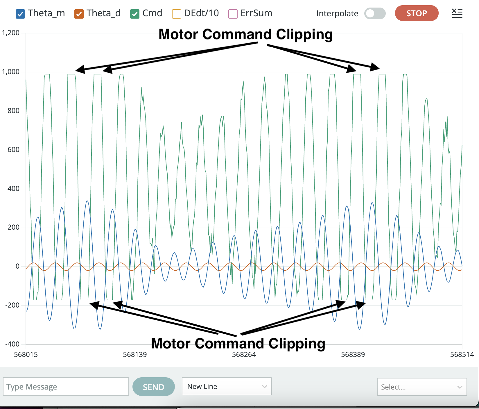
While the two-propeller arm is intended to cancel the gravity-induced nonlinearity of the one-propeller arm, the cancellation is only perfect if the arm is perfectly symmetric (so balance the arm as best you can!). In addition, there is still a "clipping" nonlinearity that arises when the controller-generated motor commands exceed power supply limitations. This nonlinearity can usually be avoided by reducing the magnitude of the sinusoidal input, provided the clipping has been detected.
Monitor the motor command plot whenever measuring frequency response, to ensure the commands are not being "clipped" by power supply limits. The clipping effect is easy to spot, as shown in the figure below. The black arrows point to cases where the motor command (the green curve) flattens, an indication that the controller's commands are being clipped because of power supply limitations.
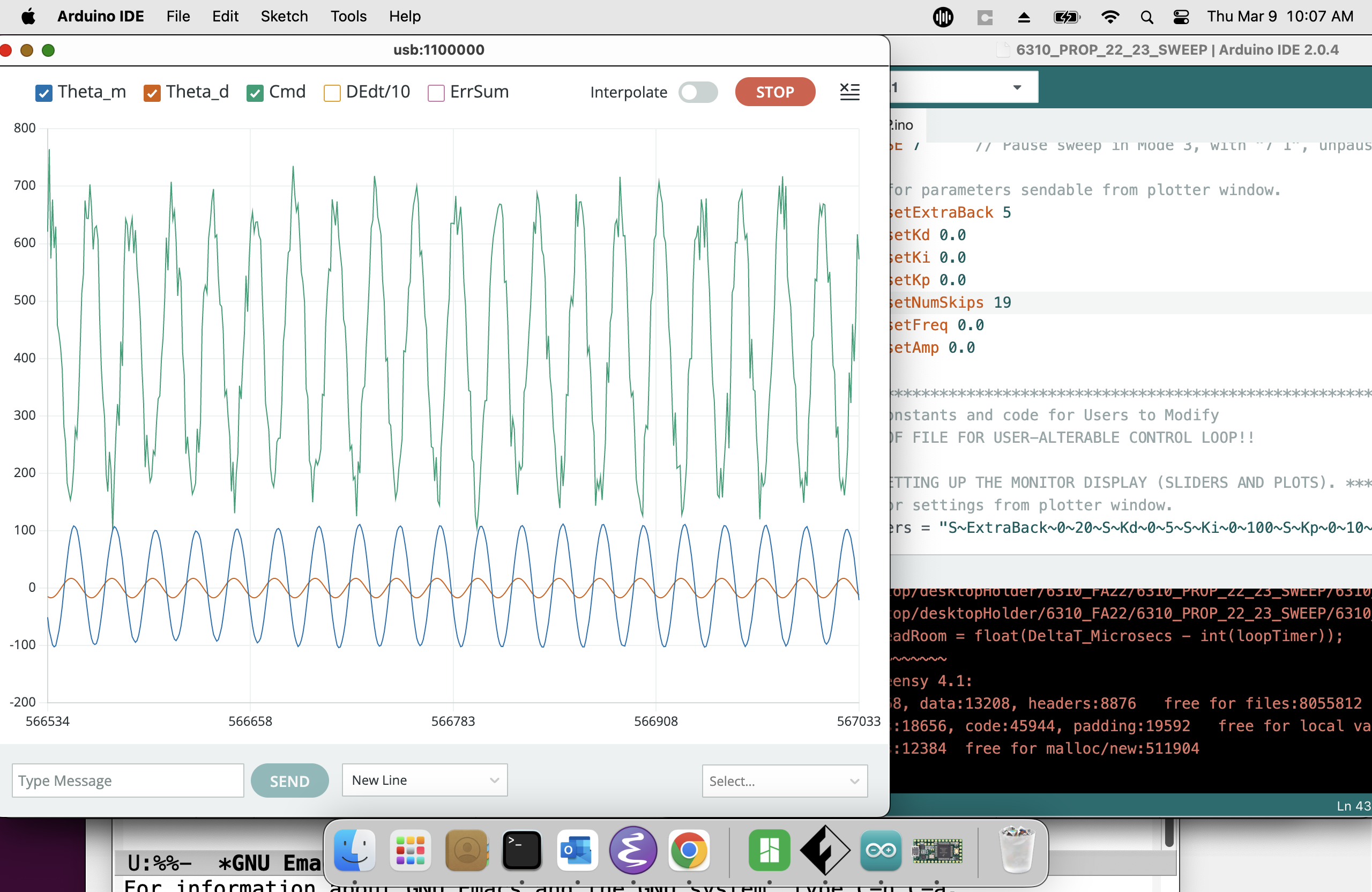
The clipping problem can usually be eliminated by reducing the input amplitude, as shown in the picture below. Avoid reducing the input amplitude too much though, because the microcontroller won't be able to represent the signal accurately. Use index 6 in the plotter window to set a reasonable sinusoidal amplitude (keep the magnitude of the amplitude at least 0.03, i.e. no closer to zero than -0.03; smaller amplitudes are not converted accurately by the controller board).
NOTE: USE NEGATIVE AMPLITUDES. THE SKETCH WILL GENERATE STEPS INSTEAD OF SINES IF YOU USE POSITIVE AMPLITUDES.
Wait for Steady-State
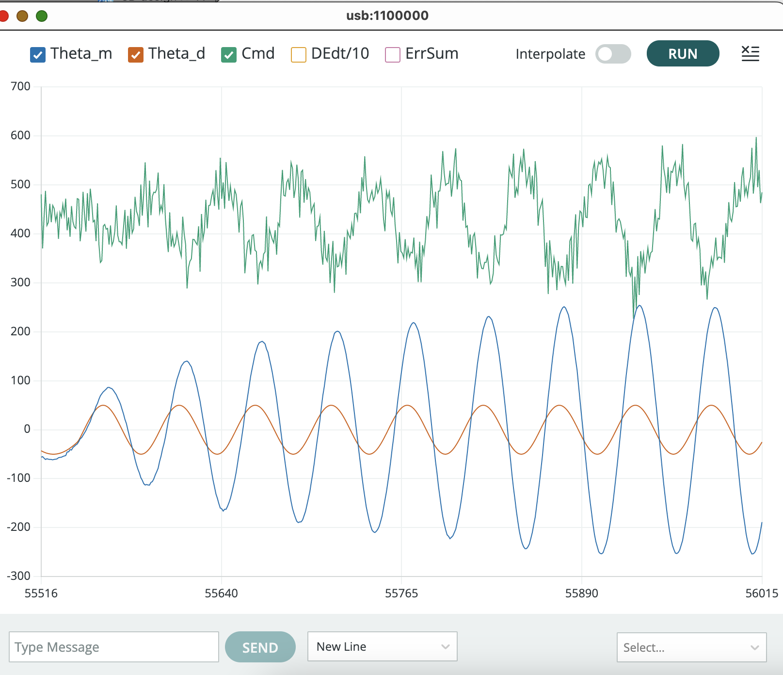
It can take several seconds to achieve sinusoidal steady-state; a typical case is shown in the picture below. Be sure to wait long enough (ten seconds or so) before pausing the plotter and taking measurements.
Spread Samples
In last week's lab, we sent an update to the serial plotter every 10 milliseconds. For this week, the sketch default is to send an update to the serial plotter every 20 milliseconds. At higher sinusoidal frequencies, it may be helpful to decrease the time between plotter updates to measure time more accurately. The control algorithm runs every millisecond, so the fastest serial plotter update is once per millisecond (zero skips). To set the fastest update rate, type "4 -19" into the plotter send window (as was done to generate the plot below). Note that the default offset for the number of skips is set to 19 in the code, and the value you send is added to that offset. As another example, to update the serial plotter every 10 milliseconds, we want to skip 9 samples, so type "4 -10" (to reduce 19 skips to 9) in the plotter send window.
Checkoff 2
For the second checkoff, please measure the frequency response of your propeller arm, with K_p=0.5, K_i=4.0 and the value for K_d you found above. You should notice that for a very narrow range of input sinusoid frequencies, the arm response increases by about five fold relative to its low-frequency response. We refer to this phenomenon as a resonance, and the center of the associated frequency range as the resonance frequency.
- Remember that the default time between plot points is twenty milliseconds.
- Measure the frequency of the oscillation in the step response.
- Measure the amplitude ratio (measured amplitude / input amplitude) and phase shift of sinusoidal steady-state responses for several input frequencies. Try to find the lowest frequency for which the phase shift is about -45 degrees (anywhere between -30 and -60 degrees is fine), and the lowest frequency for which there is a -135-degree phase shift. We suggest you use index 6 in the plotter window to set a very small sinusoidal amplitude (-0.03), because, at just the right frequency, the arm response can become quite large.
Once Again, with Feeling
Set the arm input to zero (6 0 in the send window), but do not change the feedback gains (K_i=4, K_p=0.5, and K_d is the just-barely-stable value you found in the last checkoff), and try to "fan" your system into resonance. You should be able to excite a resonance, like in the video below (an earlier version of the propeller arm was used in this video, so again, do not try to compare numerical values!!). Note that the resonance frequency for the arm in the video below is probably higher than yours, and you will try the higher resonance frequency case next. At higher resonance frequencies, it can be hard to "match" your fanning to the resonance, so please watch until (or skip to) the end to see what that looks like!!
Now try the higher resonance frequency case: set K_i=0, K_p = 2, and adjust K_d so that you get a "barely stable" step response like in the video below (an earlier version of the propeller arm was used in this video!!).
Checkoff 3
For this checkoff,
- Set K_i=4, K_p=0.5, and K_d to the just-barely-stable value you found in the last checkoff.
- TURN OFF THE INPUT, and try disturbing the arm by fanning it. Find the "fanning resonance frequency" that maximizes the response.
- Set K_i=0, K_p=2.0, and K_d to the just-barely-stable value for this no-integral-feedback case.
- Measure the frequency of the oscillation in the step response, and determine the input frequency that maximizes the sinusoidal steady-state response.
- TURN OFF THE INPUT, and try disturbing the arm by fanning it. Find the "fanning resonance frequency" that maximizes the response.
- For these two sets of controller gains, what did you observe about the relationship between the frequency of oscillations in the step response, the frequency that maximizes the sinusoidal steady-state response, and the fanning frequency that maximizes the disturbance response?
Finally, verify that you can run ipython with the control library by downloading our IPython file, ctPropArm.py, to a directory.
YOU DO NOT HAVE TO USE IPython if you prefer another python environment!!! ALSO, the file contains lines that say FIXME, do not worry about correcting those, we will address them in part B!
Open a terminal window in that directory (PowerShell on Windows, Terminal on Macs) and type ipython and return. NOT python but ipython for interactive python.
If ipython is not recognized, use pip to install ipython. Type pip install ipython followed by a return, then pip install control followed by a return. You may also need to install numpy and matplotlib using pip.
If python and pip are not installed on your laptop, but pip3 and python3 are, try the same commands with pip3 and ipython3. If that does not work, we suggest installing the Anaconda package here, but you can also install python from python.org.
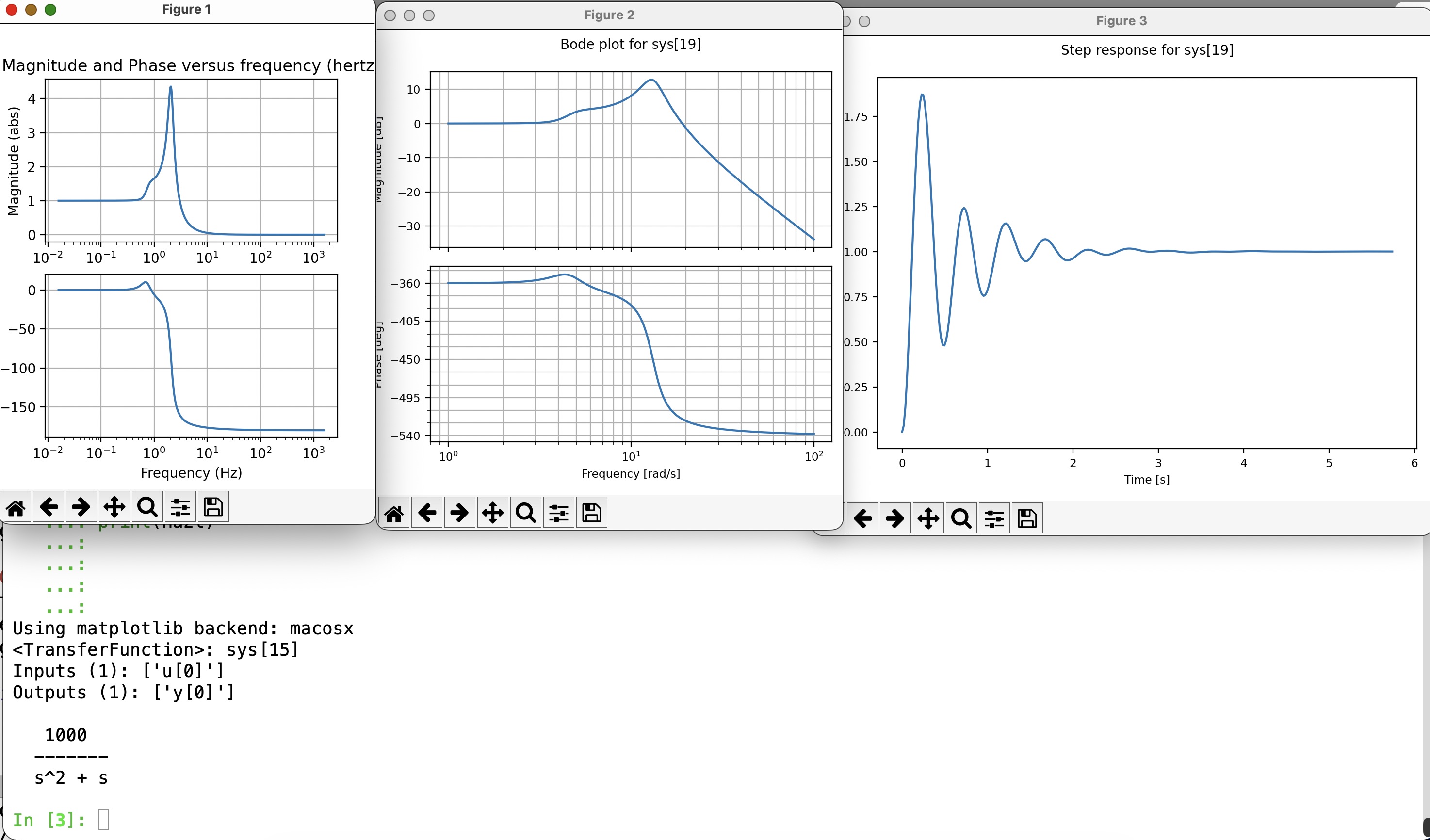
Once you have installed ipython and started it, you should get a prompt. At the prompt type %load ctPropArm.py and then press return. You should see plots and a command window like in the screenshot below.