Lab 4:
Weighting for Maglev
Please Log In for full access to the web site.
Note that this link will take you to an external site (https://shimmer.mit.edu) to authenticate, and then you will be redirected back to this page.
Quick Reference
Links
- Maglev assembly guide: here
- Sketch for this lab: 6310_MAGLEV_F26.zip
Sketch constants you will edit
| Line | Constant | Meaning |
|---|---|---|
| 11 | MODE | 0: open loop (command = input waveform), 1: PD feedback, 2: state space (later labs) |
| 12–14 | SensA, SensB, SensC | Distance-sensor fit, \Delta y = (a\,x + b)/(c\,x + 1) |
| 15 | crntSign | Sign of the field-sensor reading (set in the assembly guide) |
| 17 | Psmooth | Input-step smoothing, 0.0 (none) to 0.999 (very smooth) |
Serial plotter send-window indices
Type the index, a space and a value, then click Send (e.g.,3 4 sets K_p to 4).
| Index | Parameter |
|---|---|
| 0 | Extra samples for the derivative estimate (ExtraB) |
| 1 | Derivative gain, K_d |
| 2 | Integral gain (leave at 0 in this lab) |
| 3 | Proportional gain, K_p |
| 4 | Plot spacing (Skips) |
| 5 | Input frequency (Hz) |
| 6 | Input amplitude: >0 square wave, <0 sine, 0 none |
| 7 | Coil-current gain (state space, later labs) |
| 8 | Reference scaling, K_r (state space, later labs) |
Measuring time. The controller runs every 0.1 ms, and adjacent plotted points are (20 + \text{Skips}) \times 0.1 ms apart: 2 ms by default, or 0.5 ms after sending 4 -15.
Task Summary Part A
- Build and check the maglev by following the assembly guide (Checkoff 1).
- Calibrate the distance sensor, and find a proportional gain that makes the umbrella oscillate (Checkoff 2).
- Find a PD controller that floats the umbrella and tracks ±2 mm steps (Checkoff 3).
Introduction
In this lab and the next, you will float a "magnetic umbrella" about 1.5 cm below a three-coil electromagnet. The umbrella is a neodymium magnet in a 3-D printed holder; its top face is a diffuse infrared reflector, and its machine-screw stem keeps it from tilting, like the tail on a kite. An optical sensor measures the distance to the umbrella, a Hall-effect sensor measures the field the coils produce, and the Teensy adjusts the coil currents to keep the umbrella floating.
The video shows a previous term's system toggling the umbrella's position under a lead controller. This week you will build and calibrate the system, and find a PD controller that floats the umbrella. Next week you will model the system and use the model to design a better controller.
Strictly, this is not levitation: the umbrella hangs, it doesn't rise. But "magnetic hanging" doesn't sound nearly as cool.
Build the Maglev
Follow the maglev assembly guide from start to finish. Along the way you will:
- build the frame, electromagnet and cover bar, and wire both sensors;
- check with a compass that all three coils point the same way;
- set
crntSignso that the field reading (Crnt) follows the command (Cmd); - check the distance sensor's readings at +15 mm and −10 mm.
6 1, 5 1).

Calibrate the Distance Sensor
The optical sensor is a photo-transistor, so its reading x (the Sensor trace, between 0 and 1) grows with the infrared light reflected back from the umbrella. That light falls off steeply with distance, so x is strongly nonlinear in distance. The sketch converts x to the umbrella's displacement from its nominal position, \Delta y in mm, with the rational function
Fitting a, b and c
Multiply both sides by (c\,x + 1), and the fit becomes linear in the three unknowns:
import numpy as np
x  = np.array([0.134, 0.280, 0.560])   # readings at -10, 0, +10 mm
dy = np.array([-10.0, 0.0, 10.0])
A  = np.column_stack([x, np.ones(3), -x*dy])
a, b, c = np.linalg.solve(A, dy)
Try it first. With the example readings in the code (x = 0.134, 0.280 and 0.560), find a, b and c, and enter them as a Python list [a, b, c].
Using that fit, what \Delta y does a reading of x = 0.847 give? (That is a typical +15 mm reading.)
A fit through −10, 0 and +10 mm still predicts +15 mm well. A straight line through the same three points would not.
Taking your three readings
Set up as for the range test in the assembly guide: MODE 0, amplitude zero (6 0), only the Sensor trace plotted, the potentiometer turned so the electromagnet pulls the umbrella up, and the calibration attachment clipped on.
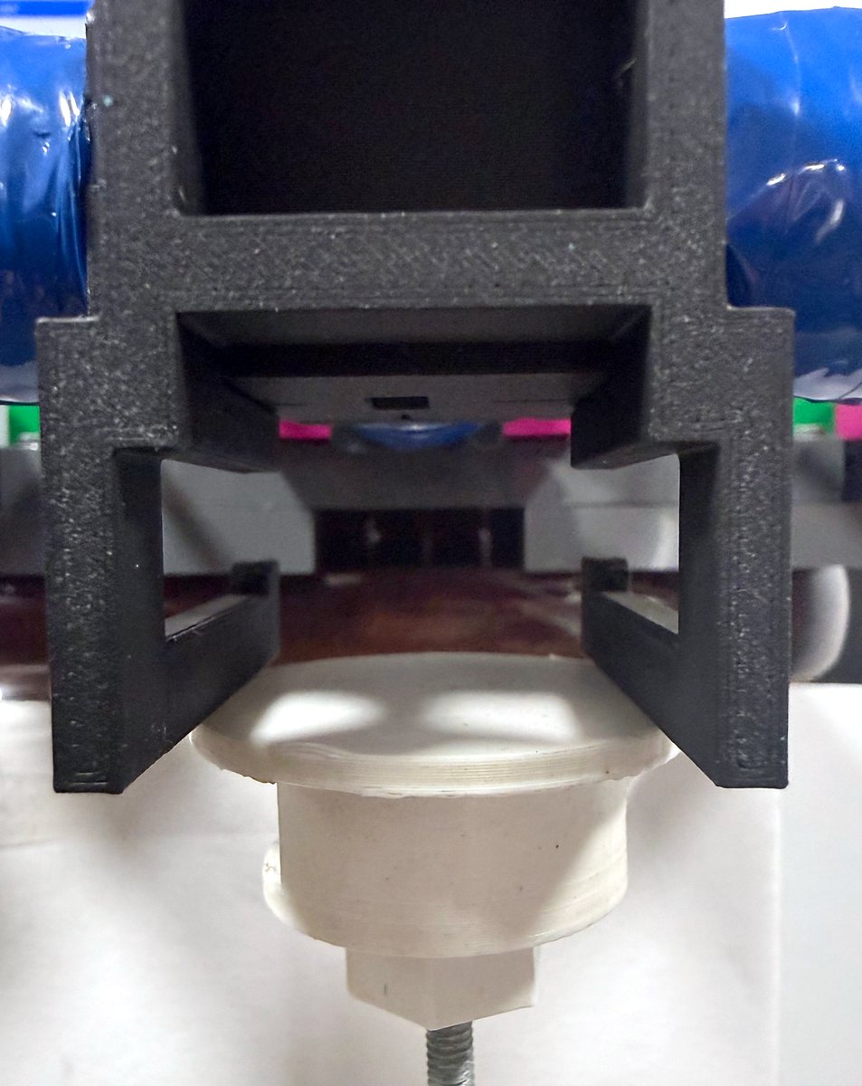
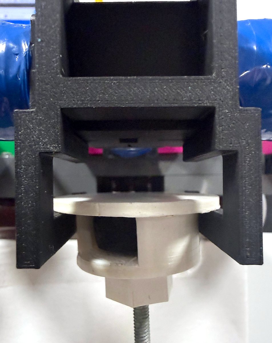
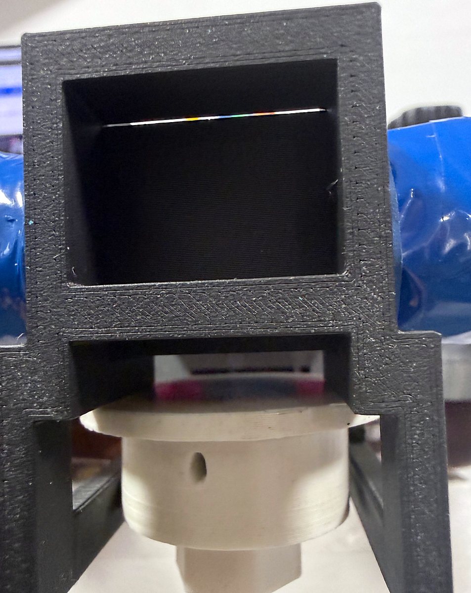
- −10 mm: use your reading from the range test.
- +10 mm: with the electromagnet still pulling up, hold the umbrella against the attachment's highest ledge, and note the reading.
- 0 mm: unplug the high-current (driver) power supply so the electromagnet is off, rest the umbrella on the attachment's middle ledge, and note the reading. Plug the supply back in afterwards.
Entering and testing your fit
- Solve for your a, b and c, enter them as
SensA,SensBandSensCon lines 12–14, and upload again. - Test the fit: remove the attachment, let the electromagnet pull the umbrella up against the sensor bracket (+15 mm), and plot Y. It should read close to 15, even though 15 mm is outside the range you fit.
Proportional Feedback
With the sensor calibrated, try feedback for the first time.
- Set
MODEto 1, upload, and set the proportional gain to 3 (send3 3). - Hold the umbrella at the 0 mm position, and turn the nominal-command potentiometer until the umbrella feels weightless: the electromagnet's pull should just cancel gravity.
- Loosen your grip. The umbrella should oscillate, at least briefly, as in the video below.
- If the electromagnet pulls harder as the umbrella gets closer, the feedback sign is wrong.
Swap the last two arguments in all three
hbridgeBipolarcalls (lines 208–210). Then also flip the sign ofcrntSignon line 15 (-1.0to1.0, or the reverse). Reversing the coil commands reverses the field the sensor sees, so without this change Crnt would no longer follow Cmd. Upload again, and recheck with the 1 Hz square wave from "Matching the Field Sensor to the Command" in the assembly guide. - If the push-back is correct but weak, increase the gain, but do not exceed 10. Higher gains saturate the coil drivers, and the system stops behaving like a linear feedback loop.
PD Control
Set MODE to 1, upload, and start from the proportional gain that made the umbrella oscillate.
Now add derivative gain K_d (index 1) to damp the oscillation.
Find a K_p and K_d that float the umbrella steadily, then test with ±2 mm square-wave steps: send 6 2 (amplitude 2 mm) and 5 0.5 (0.5 Hz).
If tracking a square wave is hard, try setting Psmooth on line 17 to 0.95.
Expect a noisy command and imperfect tracking; next week's model-based controller does much better.