Second Order Homogenous Linear Difference Equations
Please Log In for full access to the web site.
Note that this link will take you to an external site (https://shimmer.mit.edu) to authenticate, and then you will be redirected back to this page.
Crane Mutiny Example
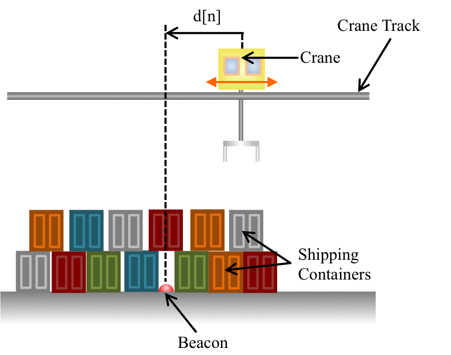
A heavy cargo crane travels on track above a buried beacon, and measures its signed distance to the beacon 100 times a second (by signed distance, we mean that the distance is positive if the crane has not yet reached the beacon and negative if the crane has traveled past it). A human operator usually drives the crane and parks it just above the beacon. The crane then keeps itself in place automatically by always accelerating towards the beacon at a rate proportional to its distance from the beacon. On one unfortunate day, the operator noticed that the crane seemed to be "rocking" back and forth over the beacon, and tried to fix the problem by flipping the sign of the distance sensor. The crane almost immediately sped off down the track, halted only by the quick-thinking operator, who shut down the crane. Why did this happen?
In the previous prelab, we assumed that we could control the crane by sending it velocity commands, which led to a first-order difference equation model. A more realistic model would be to assume that we can send the Crane acceleration commands, and that will lead to a more complicated higher-order difference equation model. We will start in the same way, and will represent the crane's measured distance to the beacon as a sequence, d, where d[n] is the n^{th} measured distance. Then d[n] can be related to d[n-1] by
There are now two sequences, v and d, and two coupled linear difference equations. As we will see below, we can use vectors and matrices to generalize many of the results from the first prelab, and use them to analyze dour Crane problem.
Matrix Difference Equations
The generic form for a vector first-order homogenous difference equation is
So what properties of \textbf{A} determine the properties of the sequence x? As we will see below, for the vector case, sequence properties are determined by the eigenvalues of \textbf{A} (assuming diagonalizability). For example, if all N eigenvalues of \textbf{A}, |\lambda_i| i \in {1,...N}, are less than one in magnitude (strictly inside the unit circle), then \lim_{n\rightarrow \infty} x[n] = 0.
To see the above result, recall that if \lambda_i is the i^{th} eigenvalue of an N \times N matrix \textbf{A}, and \textbf{V}_i is the associated N-length eigenvector, then
We can use the eigendecomposition to determine a formula for powers of \textbf{A}. For example, \textbf{A}^2 is
As the above equation makes clear, the behavior of the vector sequence x is determined by the eigenvalues of \textbf{A} just like the behavior of the scalar sequence y is determined by \lambda. For example, if \max_{i} |\lambda_i| < 1 then
Crane Example
We can write the equations for the crane as as a first-order vector equation
For a two-by-two system, we can determine the two eigenvalues using determinants, in which case the eigenvalues are the roots of the quadratic equation given by
The Crane example has complex natural frequencies, which we will return to in a later section. For now, we will stick to examples with real natural frequencies.
Fibonacci as LDE
Consider the Fibonacci sequence, in which the next element in the sequence is the sum of the previous two. The sequence has a second-order LDE description,
If we specify y[0] and y[1], which we often refer to as initial conditions, then we can use the vector difference equation to iteratively compute y[n] for all n \ge 2.
For example, to generate the classic Fibonacci numbers, set y[0] = 0 and y[1] = 1, and repeatedly apply the above formula with n =2 , then n=3, n=4, and so on, to determine y[2]=1, y[3]=2, y[4]=3, y[5]=5, ... etc. In general, given an LDE and enough initial conditions, it is easy to explicitly enumerate the rest of the sequence values.
These questions refer to the Fibonacci difference equation
- If you pick initial conditions y[0] = 8 and y[1] = 13 for the above difference equation, what will be true about the generated sequence y[2], y[3], y[4], y[5], ... ? Please list all that apply below (separated by commas).
- A: The sequence entries will grow without bound.
- B: The sequence entries match the values of a shifted Fibonacci sequence.
- C: \lim_{n \rightarrow \infty} \frac{y[n]}{y[n-1]} > 2.

Suppose the initial conditions for the difference equation are given by two constants, A and B , where y[0] = A and y[1] = B . What will be true about the generated sequence y[2], y[3], y[4], y[5], ... ? Please check all that apply.
- A: If A is negative and B is positive, and |A| \gt B , then it is guaranteed that y[n] \lt 0 for all n \gt 2 .
- B: If A is negative and B is positive, and |A| \gt 2\cdot B , then it is guaranteed that y[n] \lt 0 for all n \gt 2 .
- C: If A is positive and B is negative, and A \lt |B| , then it is guaranteed that y[n] \lt 0 for all n \gt 2 .
- D: If A is positive and B is negative, and |A| \gt |2\cdot B |, then it is guaranteed that y[n] \lt 0 for all n \gt 2 .
"Generalized" Fibonacci
Sequences described by second-order homogeneous LDEs, like the Fibonacci sequence, have the property that y[n] is given by a weighted combination of y[n-1] and y[n-2]. Their general form is
Suppose we do not know a_1 and a_2, but we do know the solution has the form
For what values of a_1 and a_2 will y[n] = a_1 y[n-1] + a_2 y[n-2] have as solution of thee form
For the following problems, consider the second-order linear difference equation
with the solution
Determine a_1, a_2, y[0], and y[1].
Matching Initial Conditions
Now that we have the two natural frequencies, there is the matter of initial conditions. How to incorporate the initial conditions is best seen by example, so we will examine solving the second-order homogeneous LDE for the Fibonacci sequence. Since the next value in the Fibonacci sequence is the sum of the previous two,
or a_1 = a_2 = 1 in our general second-order homogeneous LDE.
From the eigenvalues of the matrix \textbf{A} of the vector form of the above difference equation, we know that the Fibonacci LDE has two distinct natural frequencies,
therefore any sequence of the form
will satisfy the Fibonacci LDE.
In order to produce the classical Fibonacci sequence, we need to find values for c_1 and c_2 so that y[0] = 0 and y[1]= 1. To start, consider how y[0] = 0 constrains c_1 and c_2,
Including the constraint from y[1] = 1,
So, the final equation for the Fibonacci sequence is
Evaluating the numeric constants (approximately)


Are there values of y[0] and y[1] for which the sequence given by
decays to 0 as n approaches \infty?
Select the most accurate response below:
Consider a system modeled by the difference equation
with initial conditions y[0]=1 and y[1]=-1.
Which of the following most accurately characterizes the eventually (large n) behavior of the sequence y?