Summary and Speed Control Inconsistency

The questions below are due on Friday February 27, 2026; 10:00:00 AM.

You are not logged in.
Please Log In for full access to the web site.
Note that this link will take you to an external site (https://shimmer.mit.edu) to authenticate, and then you will be redirected back to this page.

You are viewing the PRELIMINARY 6.3100 Spring 2026 web site. Please note that information on this page may change throughout the semester, please check back frequently.

This problem is intended to give you some experience with tools used to analyze higher-order systems. In particular, we hope it will help you understand how to connect natural frequencies to time responses, and how to use root loci to determine controller gains. We will use the now-familiar motor speed control example from the first lab because, as we will clarify below, it really was a second order system. We give a very brief summary below (that you can skip until you need it).

A Naturally Brief Summary

The generic form for a zero-input N-state vector first-order difference equation is

x[n] = \textbf{A} \; x[n-1] + \textbf{B} \; u[n-1]

where x is a vector sequence whose n^{th} entry, x[n], is a vector whose length is equal to the number of states, N, \textbf{A} is an N \times N matrix, and in the single-input case, u is a sequence whose n^{th} entry, u[n], is a scalar of (typically) known value.

The solution, x[n], is a function of an initial condition vector, x[0], and the input sequence, u, and is given by

x[n] = \textbf{A}^n x[0] + \sum_{m=0}^{n-1}A^{n-1-m}Bu[m].

If the input is zero (ZIR), the above formula simplifies to

x^{ZIR}[n] = \textbf{A}^n x[0],

which is (not universally) referred to as the "natural" response, because the response is unforced by an input and is innate to the system. If \textbf{A} is diagonalizable with eigenvalues \lambda_1,...\lambda_N, we refer to these eigenvalues as "natural frequencies" because we can write the ZIR for each of the N states as state-dependent weighted combinations of these natural frequencies. More specifically, the n^{th} step of the i^{th} state is given by

x^{ZIR}_i[n] = c_{i,1} (\lambda_1)^n + c_{i,2} (\lambda_2)^n + ...+ c_{i,N} (\lambda_N)^n,

where the set of N^2 c_{i,j}'s can be determined from

{x[0], \textbf{A}x[0], ...., \textbf{A}^{N-1}x[0]},

though the set is only guaranteed to be unique if the eigenvalues are distinct (no two are equal). Since x[n] and A are real, eigenvalues are either real or in complex conjugate pairs, as are the associated weights.

It is perhaps worth noting that the eigenvalues of \textbf{A} are not always referred to as natural frequencies, with some referring to them as complex frequencies or eigenfrequencies. Using the word frequency might even seem like a misnomer, because these eigenvalues are not necessarily related to the inverse of an oscillation period. This author's perspective? These eigenvalues inhabit the entire complex plane, why worry about reserving certain words for the imaginary axis, a set of measure zero in that plane.

First Order Model for Motor Speed Control

In the motor speed control lab, Fast and Spurious, you modeled, analyzed, and measured a proportional-feedback-based motor speed control system. You extracted a first-order model of the system, and used that model to predict (fairly accurately) the stability limits on proportional feedback gains. But you also should have observed an inconsistency between the step responses associated with a first-order model and higher-order nature of the step response measurements. In this problem we will develop a second-order model of the speed control system, and show that this higher-order model not only predicts system behavior when ticksPerEstimate=8 but also explains the behavioral changes when ticksPerEstimate=1.

We modelled the speed control system with a first-order difference equation:

\omega[n] = \omega[n-1] + \Delta T \left(\gamma c[n-1] - \beta \omega[n-1]\right) \tag{1}

where \omega[n] is the motor speed (in revolutions per second, or RPS) at the n^{th} speed sample, \Delta T is the time between speed samples, \beta is a friction coefficient and \gamma is the scale factor relating microcontroller command to motor acceleration.

When the microcontroller parameter ticksPerUpdate is set to 8, the motor speed is updated once per revolution, and since the nominal motor speed is 15 rotations per second,

\Delta T = \frac{1}{15}.

The \gamma and \beta parameters were extracted from experimental data, and since no two systems were identical, those parameters varied considerably from setup to setup. To ensure this prelab is auto-gradeable, please assume the following "typical" values when solving the problems below.

\gamma = 16, \qquad \beta = 0.7, \qquad \Delta T = \tfrac{1}{15}.

The First Order Model

Assume c[n] = K_p(\omega_d[n] - \omega[n]), and write the first-order difference equation for \omega[n] in the form \omega[n] = \alpha_1\,\omega[n-1] + \alpha_2\,\omega_d[n-1]. Enter symbolic expressions (in python format) using DeltaT for \Delta T, Kp for K_p, beta for \beta, and gamma for \gamma.

Coefficient of \omega[n-1]: \;\alpha_1 =

Coefficient of \omega_d[n-1]: \;\alpha_2 =

The natural frequency, \lambda, of this first-order system is

Natural frequency: \;\lambda =

Given the values of \beta and \gamma above, and assuming \omega_d[n] = 0 for all n and \omega[0] = 1, find a value for K_p so that \omega[n], n = 0,1,2,3,4,5,6 oscillates at least twice, and that \omega[6] = 0.5. Please first determine the value of \lambda, (careful about signs!) and then determine the seven values of \omega[n], for n = \{0,1,2,3,4,5,6,7\}.

What \lambda produces the above decay (enter a number):

Enter your seven values, \omega[0], ...\omega[6] as a python list in answering the question below. A lollipop plot of your sequence will appear right after you click the submit button.

Enter [x[0],\, x[1],\, \ldots,\, x[6]] as a Python list:

The Second Order Model

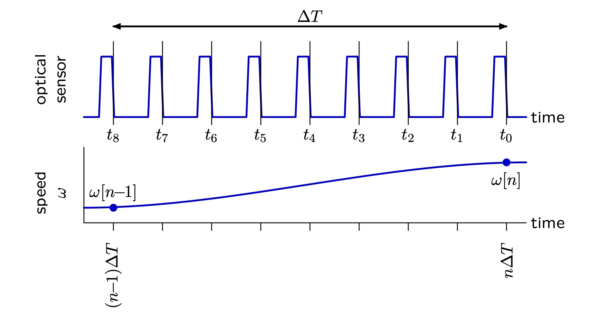
The speed control hardware does not measure \omega directly. Instead, the speed is estimated from timing pulses generated by reflections from the eight-bladed propeller spinning beneath an led-sensor pair. Using the notation in the figure below, which shows the timing when ticksperupdate=8 and ticksperestimate=8.

For the case shown below, the sampling interval is \Delta T = t_0 - t_8, and the associated motor speed estimate \widetilde{\omega}[n] is given by \widetilde{\omega}[n] = \frac{1}{t_0-t_8}.

In the first order model, we assumed

\widetilde{\omega}[n] = \frac{1}{t_0-t_8} \approx \omega[n],

but \widetilde{\omega}[n] is a more accurate approximation to the average of \omega[n] and \omega[n-1] as in

\widetilde{\omega}[n] = \frac{1}{t_0-t_8} \approx \frac{\omega[n]+\omega[n-1]}{2}.

Given the above insight, a more accurate description of speed controller is:

c[n] = K_p \left(\omega_d[n] - \frac{\omega[n]+\omega[n-1]}{2}\right),

which when substituted into (1) (and collecting terms) yields a second-order difference equation:

\omega[n] = \!\left(1 - \beta\Delta T - \tfrac{1}{2}\gamma K_p\Delta T\right)\omega[n-1] - \tfrac{1}{2}\gamma K_p\Delta T\,\omega[n-2] + \gamma K_p\Delta T\,\omega_d[n-1]. \tag{2}

Matrix Form

We can rewrite equation (2) in matrix form by creating a vector from the n^{th} and (n+1)^{th} samples of motor speed as in

\begin{pmatrix}\omega[n]\\\omega[n-1]\end{pmatrix} = A\begin{pmatrix}\omega[n-1]\\\omega[n-2]\end{pmatrix} + B\,\omega_d[n-1].

Please give formulas for each entry in the A matrix and B vector as a symbolic Python expression, using DeltaT for \Delta T, Kp for K_p, beta for \beta, and gamma for \gamma.

A_{11} =

A_{12} =

A_{21} =

A_{22} =

b_1 =

b_2 =

Natural Frequencies (eigenfrequencies)

What are the natural (eigen)-frequencies (eigenvalues of A) of our second order model of the speed controller? We could try to compute them as analytic functions of the gain, K_p, and for a second-order (and even third-order) models, it is possible to determine closed form analytic expressions, but not for higher order models (there is no closed-form general formula for the roots of polynomials above order three, or for eigenvalues of square matrices of dimension higher than three). Instead, we can plot a root-locus of natural frequencies for a range of parameters, and use those plots to determine properties of interest.

The question below is not really a question, but rather a tool (so it always grades as correct) for plotting root-loci and associated time responses. Specifically, the tool plots the eigenvalues of A({K_p}), as K_p varies over a given range. The tool also plots a pair of ZIR's, ones associated with the largest and smallest values of the specified range of K_p's.

Please enter the 2 \times 2 matrix A(K_p) as a Python nested list with entries as analytic functions of ONLY K_p (so please substitute the numerical values given above for \beta, \gamma and \Delta T), and please represent K_p using the python variable Kp. Finally, please follow the matrix specification with the gain range and number of plotting points using the format

Kp=[lowKp,highKp], n=[nstart,nStop].

As an example (NOT THE CORRECT MATRIX!! NOT THE CORRECT MATRIX! NOT THE CORRECT MATRIX!), if the matrix for our system was

A(K_p) = \begin{bmatrix} 1 & 1 \\ -2K_p & 0 \end{bmatrix}

and we wanted to examine the natural frequencies and twenty points of the ZIR for values of K_p that range from zero to 5, we could answer the question below with

[[1, 1],[-2*Kp, 0]], Kp = [0,0.5], n=[0,20]

Plotting Tool.

A(K_p), params:

Use the plotting tool above to find the LARGEST K_p for which the magnitude of the maximum-magnitude eigenvalue is less than 0.9. ADVICE: the above root locus plot will be easier to interpret if you set the high end of the gain so that

max|\lambda\left(\textbf{A}(highKp)\right)| \approx 0.9.

Please use observations from our root-locas plotter to answer the questions below.

What value of K_p gives a maximum-magnitude eigenvalue of approximately 0.9? (within 15%)

What is the angle (in degrees) of the maximum-magnitude natural frequency at that K_p?

Approximately how many samples are in one oscillation period at that K_p? (360^\circ / |\text{angle}|)

Reducing the Measurement Delay

The ticksperestimate=8 estimate uses the full motor rotation t_0-t_8 to estimate the motor speed, introducing a kind of delay. Instead, we could set ticksperestimate=1, in which case

\hat{\omega}[n] = \frac{1/8}{t_0 - t_1}

As before, we relate this to \omega[n] and \omega[n-1] by linear interpolation:

\hat{\omega}[n] = a\,\omega[n] + b\,\omega[n-1], \qquad a+b=1,\quad a\ne\tfrac{1}{2}

What are the numerical values of a and b?

a =

b =

Using a and b above, update the formulas for the entries of A and B using a, b, DeltaT, Kp, beta, gamma.

a_{11} =

a_{12} =

a_{21} =

a_{22} =

b_1 =

b_2 =

Use the plotting above to find a value for K_p so that the magnitude of the maximum magnitude natural frequency is approximately 0.9.

What value of K_p gives a maximum-magnitude eigenvalue of approximately 0.9? (within 15%)

What is the magnitude of the angle (in degrees) of the maximum-magnitude natural frequency at that K_p?

Approximately how many samples are in one oscillation period? (360^\circ / |\text{angle}|)

The behavior of the controller using the reduced delay motor speed estimate was much closer to the behavior predicted by the first-order model, do you see why?