Dynamical System Modeling and Control Design
Please Log In for full access to the web site.
Note that this link will take you to an external site (https://shimmer.mit.edu) to authenticate, and then you will be redirected back to this page.
Welcome to Dynamical System Modeling and Control Design -- Fall 2022
Find syllabus, lab descriptions, and assignments by following the calendar and handouts link on the above "Information" tab, find software installation info, lab assembly instructions, and help queue information on the "Resources" tab.
Please join live lectures, MW3-4, 4-231, and live lab sessions, F10-1 or 2-5, 38-545. Lectures will be recorded, and can be found at Lectures.
Have you ever wondered about the control strategies used temperature regulators, quad-copters, aircraft autopilots, self-driving cars and agile robots? Are you curious about the policies that govern flow in large networks, like the web or the electric power grid? Or are your interests more biological, and you want to know how the body maintains balance, regulates glucose, or repels infection? Or maybe you used a PID controller in a robotics competition, and are now ready to learn more?
If so, you are interested in the general topic of feedback control, in which sensor data (e.g. brightness, temperature, velocity, location, etc.) is used to adjust or correct actuation (e.g. steering, acceleration, or heater output). And yes, as the above examples make clear, feedback control is ubiquitous. But, it is also a uniquely compelling example of mathematical theory guiding practical design. In 6.3100/2 class, we will focus on introducing you to this beautiful marriage of theory and practice, and try to give you a framework for further study, by focusing on a small set of key concepts, which we will apply to controlling several different physical artifacts.
6.3100/6.3102 -- The lab kit.
KITS ARE SELF-CONTAINED: So 6.3100/6.3102 can be continued remotely if needed.
The core of the lab kit is our PC board with a high-performance microcontroller, four pulse-width modulated drivers, eight buffered analog inputs, and four buffered analog outputs. The microcontrollers are easily programmed with a version of the widely-used Arduino environment, sensors and actuators are easy to connect, and your laptop can monitor and allow you to make adjustments in real time (you can even turn your laptop into a rudimentary oscilloscope). With the PC Board, a kit of parts (which includes motors, coils, sensors, propellers,lego, and 3-D printed connectors), a laptop, and our additional software, you will be able to build a variety of interesting artifacts, control them with a variety of approaches, and EASILY run experiments and collect data.
We think students who work together in pairs, join us for lectures, and attend lab periods in person, will have the best experience. But, we are committed to making sure that everyone can participate. The 6.310/6.3102 PC board and a kit of parts (plus your laptop) is a self-contained lab, we will record our lectures, and we can be available for zoom-based help, lab check-offs, and interviews.
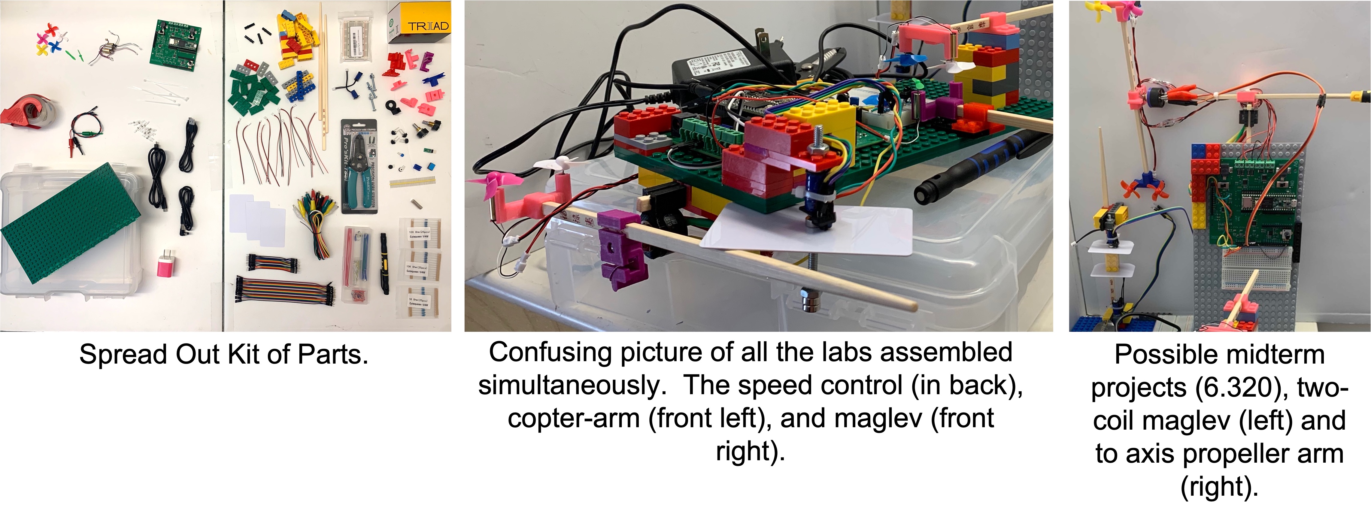
The left picture above is a spread of all the parts in the lab kit (from last fall, is being updated). As you can sort of see, there are motors, propellers, coils, nuts and bolts, optical distance sensors, jumpers, Lego parts, Lego-compatible 3-D printed parts, a high-current power supply, a USB to microUSB cable and a USB-C to microUSB cable, a wire stripper, and a screwdriver. The middle picture above shows the parts assembled into three artifacts at once: an optical sensing speed controller (the green propeller over an optical sensor, barely visible in the back), a double-propeller rotating arm (front left), and a magnetic levitator (with the magnets and white reflecting card stuck to the coil bolt in the front right). In the left picture in the back are extra parts for possible midterm projects (a two-coil floating cylinder, and a two-axis arm). The artifacts are shown in a little more detail, and in action, below.
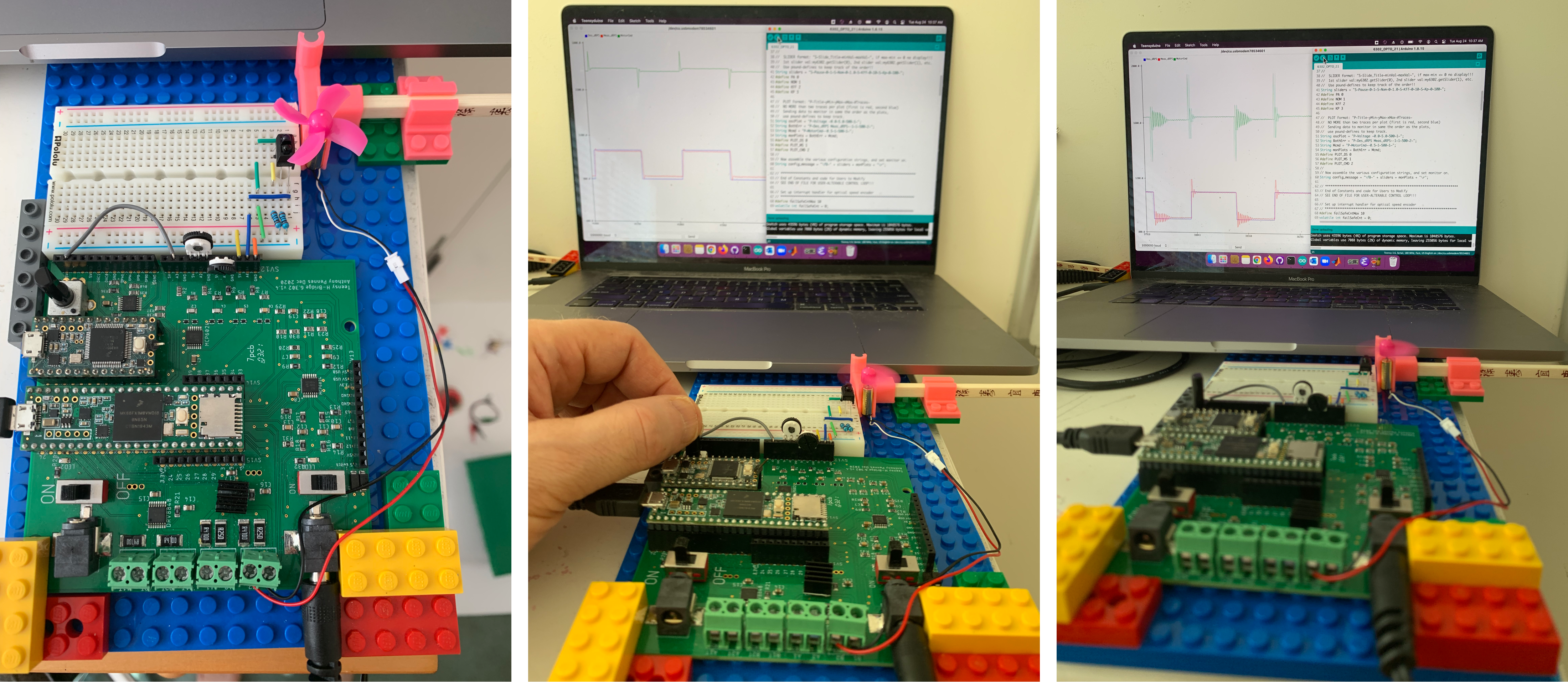
In the left picture above, we show a snapshot of a system that uses proportional-feedback to control the speed of a propeller. The leftmost picture shows the system: a motor that spins a four-blade propeller above an optical sensor, and a microcontroller board which reads the sensor and drives the propeller motor. In the middle and right pictures, the laptop displays a graph of the motor command above the desired and measured rotation speeds, with the middle picture showing low feedback gain, and the right showing higher gain. As the middle and rightmost plot (of the measured and desired speeds) shows, the desired propeller speed is being toggled between 100-10 and 100+10 RPS, and the measured (or actual) speed of the propeller is tracking (mostly) the toggling of the desired speed. Please take particular note of the "overshoot" in the propeller's measured RPS in the rightmost picture. That is, when the desired speed changes from 90 to 110 RPS, the measured speed exceeds 110 RPS but eventually "settles down" to the correct value. You'll come to understand why this overshoot occurs, and more importantly, will know how to change the sensing and the control to improve the system's performance, by the end of the second week of 6.310/6.3102.
The above picture shows the same microcontroller and software system running a two-axis propeller-driven arm, one of the possible midterm projects. Below are videos of some of the more advanced labs and projects.
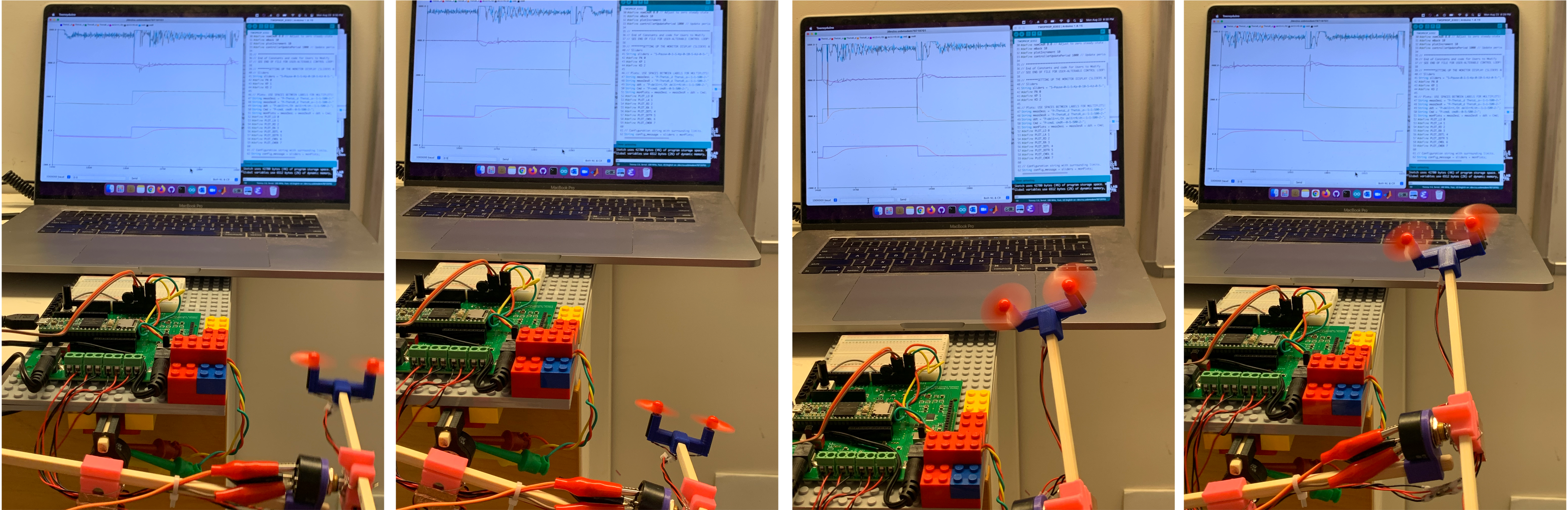
On the left are two magnetic levitation control systems in action, in which pairs of electromagnets are holding either a cylinder or bar, with permenant magnets attached, suspended and moving up and down or tilting in space. Notice that the laptop is displaying both control systems (cylinder on top and bar on the bottom). That is, every second or so, the cylinder moves up or down, and the bar tilts back and forth. On the right is a two-propeller arm, being controlled using a state-space based approach. Note that the arm is taking steps from -2 to 2 radians (or rotating about 230 degrees), and that three plots of the system behavior are being displayed on the laptop screen. If you look carefully at the leftmost of the three plots, which shows rotation angle, while watching arm rotation, you can see angle "overshoot" in both. That is, the arm rotates a little too far and then corrects itself. By the end of this class, you will be able to eaily design a much better state space controller.
6.3100/6.3102 FAQ
What is a typical week in 6.310/6.3102?
Is 6.310/6.3102 too advanced? Or too elementary?
How is 6.310/6.3102 graded?
What class hours are required?
What are the final checkoff interviews?
Each of the final lab checkoff interviews are one-on-one, but are pass/retry(without penalty). We do these interviews individually because we try to tailor the interview to each student. So, we expect many of the first tries at these one-on-one interviews will involve untangling some confusions, but will be followed by second try interviews that demonstrate more thorough mastery. But we will also try to extend the understanding of even the best prepared students, so that every student learns something in every interview, and the experience is never just "box-checking".
Will there be an open-ended project?