First Order Examples: Root Locus and Linearization

The questions below are due on Friday September 15, 2023; 09:59:00 AM.

You are not logged in.
Please Log In for full access to the web site.
Note that this link will take you to an external site (https://shimmer.mit.edu) to authenticate, and then you will be redirected back to this page.

Velocity-Controlled Crane

Crane traveling on a track and measuring distance to a Beacon.

Crane proportional controller.

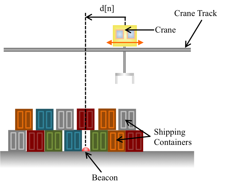
In the Crane example, recall that the distance from the beacon for the velocity-controlled crane, in Figure 1, is described by the difference equation

d [n] = d [n - 1] + Δ T \cdot v [n - 1],

where

d [n]

and

v [n]

are the

n^{t h}

measured distance and controlled velocity respectively. Recall also that if we use the controller as diagrammed in Figure 2 with proportional feedback, then the velocity is given by

v [n] = K_{p} (d_{d e s} [n] - d [n]) .

where

K_{p}

is the proportional gain and

d_{d e s}

is the desired position.

LDEs for distance and error

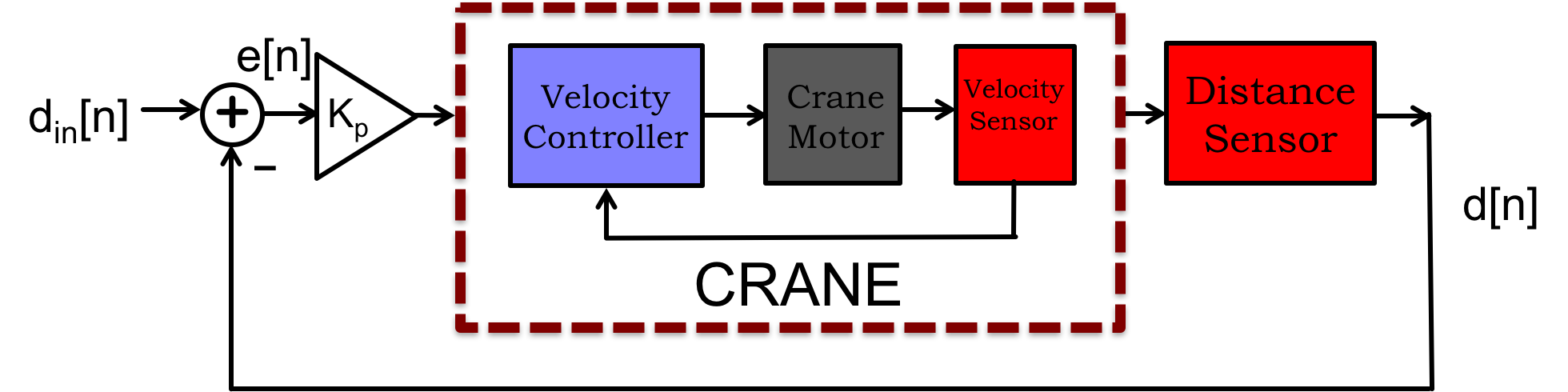
The model for the Crane, the first of the equation pair above, and the crane controller, the second of the pair, are both linear difference equations (LDEs). Whenever possible, we prefer LDE models of systems we want to control, mostly because we have so many good analysis tools for LDEs. For example, the model and controller LDE's for the Crane can be merged into a single difference equation,

d [n] = (1 - Δ T \cdot K_{p}) d [n - 1] + Δ T \cdot K_{p} \cdot d_{d e s} [n - 1],

a first-order LDE with natural frequency

λ = (1 - Δ T \cdot K_{p})

and input

d_{d e s}

We can also write an LDE for the "error", $e [n]$ , defined as the difference between the actual and desired crane position,

e [n] \equiv d_{d e s} [n] - d [n] .

The LDE for the Crane position error is easily derived by subtracting the crane model equation from the equation $d_{d e s} [n] = d_{d e s} [n]$ , then merging the result with the controller eqation, and finally substituting in the definition of the error. That is, subtracting yields

d_{d e s} [n] - d [n] = d_{d e s} [n] - (d [n - 1] + Δ T \cdot v [n - 1]),

and then merging and substituting yields

e [n] = e [n - 1] - Δ T \cdot K_{p} \cdot e [n - 1] + (d_{d e s} [n] - d_{d e s} [n - 1]) = (1 - Δ T \cdot K_{p}) e [n - 1] + (d_{d e s} [n] - d_{d e s} [n - 1]) .

The error equation is particularly simple when if the desired input stops changing. That is, if

(d_{d e s} [n] - d_{d e s} [n - 1]) = 0

for

n > N

, then

e [N + n] = (1 - Δ T \cdot K_{p})^{n} e [N],

so the error goes to zero as

n \to \infty

∥ (1 - Δ T \cdot K_{p}) ∥ < 1

In deriving the error equation, notice that we have used a small trick, adding and subtracting $d_{d e s} [n - 1]$ , as in

d_{d e s} [n] - d [n - 1] = d_{d e s} [n] - d_{d e s} [n - 1] + d_{d e s} [n - 1] - d [n - 1] = d_{d e s} [n] - d_{d e s} [n - 1] + e [n - 1] .

Crane Root Locus

Natural frequencies are innate to a system, so are invariant to changes in variables. For example, the nature frequency of the first-order LDE describing the feedback-controlled crane, $λ$ , is the same regardless of whether the system is described as a difference equation in distance, $d [n]$ , or a difference equation in error, $e [n]$ . That is, for either difference equation,

λ = (1 - Δ T \cdot K_{p}) .

When determining gains for a control system, it can be helpful to have a plot of how the natural frequencies change with changes in feedback gains. Such plots, usually referred to as "root-locus" plots, are often easier to generate than an explicit functional relationship between gains and natural frequencies. More on this when we discuss higher-order difference equations. It is also true that root-locus plots can lend more insight, even in the first-order case. We show such a plot of natural frequency versus gain in the figure below.

The points in the plot below are the natural frequencies for different gains in the Crane system. Note that the plot shows the natural frequencies as points in the complex plane (x-axis for real, y-axis for imaginary), even though they are real for first-order systems. As we will see once we start examining second-order systems, natural frequencies are the roots of a system-specific polynomials, and are general are complex. Also, we refer to the plots like Figure 3 as a root-locus plots, because the curves in the plots are formed from the "locus" of roots of the polynomials generated by sweeping a system's feedback gain from zero to infinity. Finally, root-locus plots for discrete-time systems often explicitly denote the unit circle $| λ | = 1$ , because a system with a natural frequency outside the unit circle is unstable.

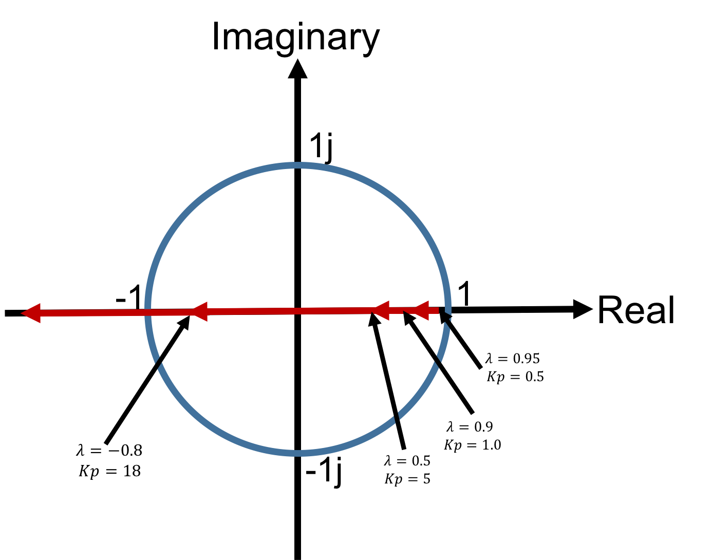
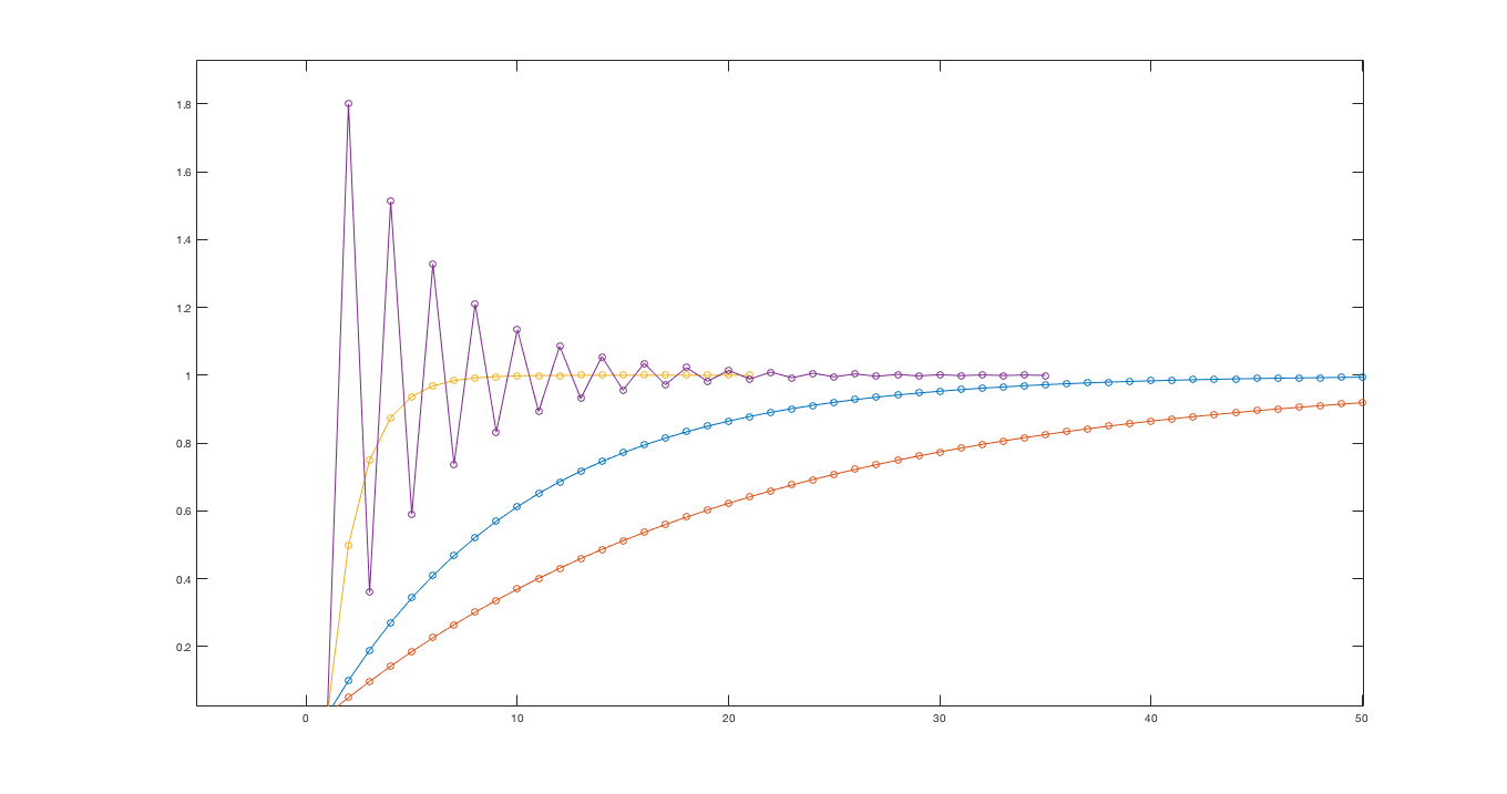
Root Locus For Crane with Velocity control.

The arrows in the red curve of Figure 3 show the path of the natural frequency with increasing gain. As the plot shows, with increasing gain, the natural frequency moves from close to one, towards zero, then towards negative one, and finally outside the unit circle. The step responses for the system, in Figure 4, show the same trend with increasing gain. As the gain rises, the transient becomes faster and faster as the natural frequency approaches zero, and when it passes zero and becomes negative, the step response becomes oscillatory. For even larger gains, the system becomes unstable.

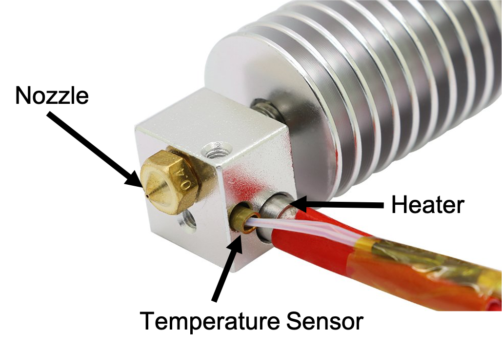
Step responses for the gains shown in the root locus plot above. Note the osillating response associated with the negative natural frequency with high gain.

A thermal example

Most fused-filament 3-D printers "print" by extruding melted plastic filament through a temperature-controlled nozzle, like the one on the 3-D printer "hot-end" shown below. Along with the nozzle, the "hot-end" includes a heater, a temperature sensor, and large metallic "heat sink". The heat sink conducts heat away from the filament path, and insures that the high nozzle temperature will not lead to melting of the plastic filament before reaching the nozzle. Keeping the nozzle at a fixed high temperature given the high rate of heat conduction is a challenging problem, particularly given the variability in ambient room temperature.

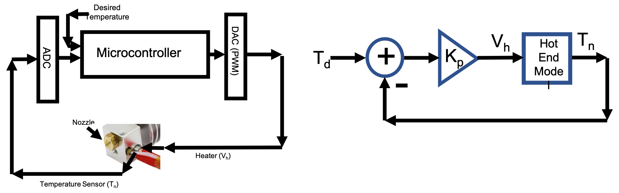
A 3-D printer hotend, showing nozzle with temperature sensor and heater.

Suppose we wish to design a feedback control system for the hotend, one that keeps the nozzle at $T_{n}$ by adjusting the voltage, $V_{h}$ on the nozzle heater based on measurements from the nozzle temperature sensor. A diagram of the connections and the mathematical block diagram is shown in the figure below.

A 3-D printer hotend and controller. On the left, the hotend and the microcontroller diagram, on the right, the control system block diagram.

A very simple model

A simple model relating the voltage on the heater to the nozzle temperature can be derived by relating the net heat flowing into the nozzle to the rate at which the nozzle temperature changes. Assuming the nozzle heater is lossless, the heat it generates is equal to the applied electric power, which in turn is equal to the product of heater voltage and electric current. And since the electric current is equal to the heater voltage divided by its resistance, the applied power, and therefore the generated heat, depends quadratically on voltage. That is,

\approx V_{h} \cdot I_{h} = \frac{(V_{h})^{2}}{R} .

where

R

is the heater resistance.

Heat flows into the nozzle from the the heater, but also flows out from the nozzle, conducted by the heat sink into the external environment. Conductive heat loss is typically proportional to the difference between nozzle and ambient (or external environment) temperature, as in

\approx - β (T_{n} - T_{a}) .

In the above equation,

T_{a}

is the ambient (or external environment) temperature and

β

is an effective thermal conductivity for the heat sink.

If we are sampling the nozzle temperature every $Δ T$ seconds, and if we assume that the change in temperature is equal to net heat flow (scaled by the heat capacity of the hot end) then a simple NONLINEAR difference equation for the sampled nozzle temperature is

T_{n} [n] \approx T_{n} [n - 1] + \frac{1}{C} Δ T \cdot (- β (T_{n} [n - 1] - T_{a}) + \frac{(V_{h} [n - 1])^{2}}{R}) .

where

T_{n} [n] \approx T_{n} (n \cdot Δ T)

, and

C

is the heat capacity of the hot end.

Linearizing

If the heater voltage is held constant at $V_{h_{0}}$ , then the steady-state nozzle temperature $T_{n_{0}} = l i m_{n \to \infty} T_{n} [n]$ can be determined by balancing the heat generation and loss. That is, given $V_{h_{0}}$ , $T_{n_{0}}$ can be found by solving the nonlinear flow-balance equation,

- β (T_{n_{0}} - T_{a}) + \frac{(V_{h_{0}})^{2}}{R} = 0.

Suppose we are designing a control system that adjusts heater voltage to maintain a specified, or desired, nozzle temperature, $T_{n_{0}}$ . Since we know a lot about analyzing first-order LDEs, perhaps we can gain insight into the control system's performance by first linearizing the system about $T_{n_{0}}$ (and its associated $V_{h_{0}}$ ), and then analyzing the resulting LDE.

A short digression: In our thermal example, there is only one nonlinearity, the quadratic relation between voltage and heat generation. Linearizing in this case is therefore equivalent to replacing the quadratic voltage-heat relation with its first-order Taylor series expansion. But are we justified in dropping the second-order term in the Taylor series? That is, will our analysis of a linearized model accurately predict the behavior of the nonlinear system? In general, the answer is an unequivocal..maybe. But if the system is first order, and if the linearized system's natural frequency is strictly less than one in magnitude, and if the system is never perturbed too far from the linearization point, then yes. We will use linearization in this class quite often, but a comprehensive treatment of its limitations is both fascinating and well beyond our scope.

Back to deriving the linearized LDE. To start, we will use lower case letters to denote the perturbations from steady state. That is,

t [n] = T_{n} [n] - T_{n_{0}} v [n] = V_{h} [n] - V_{h_{0}} .

Assuming the pair $T_{n_{0}}, V_{h_{0}}$ satisfy the heat flux balance equation above, then we can use first order Taylor expansions to write an LDE that relates the perturbed quantities, $t [n]$ to $v [n]$ as

t [n] \approx t [n - 1] + Δ T \cdot (α t [n - 1] + γ v [n - 1]),

where

α

and

γ

are related to

β

R

C

V_{h_{0}}

and

T_{n_{0}}

. And once we have the LDE model based on perturbation, we can add a proportional gain controller,

v [n] = K_{p} \cdot (t_{d} [n] - t [n]),

and use all of our analysis tools for first order systems to determine disturbance rejection, stability limits on

K_{p}

, etc. Note that here,

t_{d}

is a desired perturbation in temperture, but is likely to be zero (because we are trying to hold the temperature equal to

T_{n_{0}}

Uhm, well, perhaps our statement "we can use first order Taylor expansions to write an LDE relating perturbed quantities..." was a little glib, and we should look at the steps involved. We can start by subtracting $T_{n_{0}} = T_{n_{0}}$ from the nonlinear difference equation model (along with one of our favorite tricks, used above, where we strategically add $- T_{n_{0}} + T_{n_{0}}$ ),

T_{n} [n] - T_{n_{0}} = T_{n} [n - 1] - T_{n_{0}} + \frac{1}{C} Δ T \cdot (- β (T_{n} [n - 1] - T_{n_{0}} + T_{n_{0}} - T_{a}) + \frac{(V_{h} [n - 1])^{2}}{R}) .

Next, we use the definitions of

t [n]

and

v [n]

to get

t [n] = t [n - 1] + \frac{1}{C} Δ T \cdot (- β (t [n - 1] + T_{n_{0}} - T_{a}) + \frac{(v [n - 1] + V_{h_{0}})^{2}}{R}) .

We can using a first order Taylor expansion of

v [n - 1]

in the nonlinear heat generation term

(v [n - 1] + V_{h_{0}})^{2}

(v [n - 1] + V_{h_{0}})^{2} \approx 2 V_{h_{0}} * v [n - 1] + (V_{h_{0}})^{2},

and then take advantage of the fact that

- β (T_{n_{0}} - T_{a}) + \frac{(V_{h_{0}})^{2}}{R} = 0,

to arrive at the values for

α

and

γ

in our perturbed system LDE.

Are the rest of the steps clear? If so, what are $α$ and $γ$ as a function of $β$ , $C$ , $V_{h_{0}}$ and $T_{n_{0}}$ . In answering the questions below, give your expression as a legal python expression and use B for $β$ , R for $R$ , C for $C$ , V0 for $V_{h_{0}}$ , and T0 for $T_{n_{0}}$ . Be careful about signs, and use appropriate parentheses, when dividing by products. So the reciprocal of product of $V_{h_{0}}$ and $T_{n_{0}}$ should be written as 1/(V0*T0).

alpha =

gamma =

In our temperature model, the terms involving temperature where all linear. Does that explain why $T_{n_{0}}$ did not explicitly appear in the equations for $α$ and $γ$ ?