Lab 10 Supplement

You are not logged in.
Please Log In for full access to the web site.
Note that this link will take you to an external site (https://shimmer.mit.edu) to authenticate, and then you will be redirected back to this page.

This prelab is intended to be a little extra practice on frequency response plots, poles and zeros, step responses, and phase margin, to help solidify your understanding while you work on the CCMM lab.

State space will begin with a short pre-prelab next week, and a more serious prelab the week after, followed by the first of two state-space labs.

Quick Tour: Matlab Tools for CT and Frequency Response.

You can use matlab to manipulate continuous-time transfer functions, but there are a few differences between s- and z-domain manipulation. First, you have to tell matlab to use s as the CT transform variable, by typing

>> s = tf('s')

After that, you can define a CT transfer function. For example, suppose your system is described by a set of differential equations

\frac{d v(t)}{dt} = x(t), \;\;\; \frac{d w(t)}{dt} = v(t), \;\;\; \frac{d y(t)}{dt} = -0.1y(t) + w(t),

then assuming y(t) = Y e^{st} and x(t) = Xe^{st},

Y = \frac{1}{s+0.1}\frac{1}{s}\frac{1}{s} X = H(s) X,

where H(s) is the CT transfer function given by

H(s) = \frac{1}{(s+0.1)s^2}.

In matlab, if you type

>> H = (1/(s+0.1))*(1/s)*(1/s)

Matlab will response with

H =
 
        1
  -------------
  s^3 + 0.1 s^2

Then if you type

>> pole(H)

matlab will respond with

as you would expect since in CT, two of your poles are at zero.

Many of the matlab commands you've used before translate in the obvious way (feedback, step, etc), and we will also make extensive use of the bode command

bode(H)

For example, consider a system with input x(t) and output y(t) described by a first-order differential equation,

\frac{d y(t)}{dt} = -y(t) + 1000 x(t),

where y is the output and x is the input. Suppose we know that x(t) = \cos(\omega t) = \cos(2\pi f t) where \omega is the frequency in radians per second and f is the frequency in cycles per second. Approximately what is y(t) in the limit as t \rightarrow \infty ?

In this case, the system function is H(s) = \frac{1000}{s+1}. We say x(t) is equation to a unit step if x(t)=0 for t < 0, and x(t) = 1 for t \ge 0. To plot the response to the unit step using matlab, in the command window type (be sure you have defined s to matlab using s = tf('s')).

H = 1000/(s+1)

to define the system function to matlab, and then

step(H)

to plot y(t) given x(t) is a unit step. Note that y(t) rises to 1000 with a time constant of one second (about two-thirds of the rise in one second).

The frequency response of this first-order system can be plotted using

bode(H)

A Bode plot with the unity-gain |H(j\omega)|=1 frequency and phase margin denoted can be plotted using

margin(H)

If we use feedback with this first order system, so that

X = K(s) (Y_{desired} - Y),

then we can apply Black's formula to determine the closed-loop system function, G(s),

G(s) = \frac{K(s)H(s)}{1 + K(s)H(s)} .

If we set K(s) = 1, then

G(s) = \frac{1000}{s+1001}.

We can also use matlab to determine the system function with the feedback command,

G = feedback(1000/(s+1),1)

In order to plot the locus of poles of G(s) as a function of K_0 of

G(s) = \frac{K_0 K(s)H(s)}{1 + K(s)H(s)} = \frac{1000K_0}{s+1001},

you can use the root locus command

rlocus(1000/(s+1))

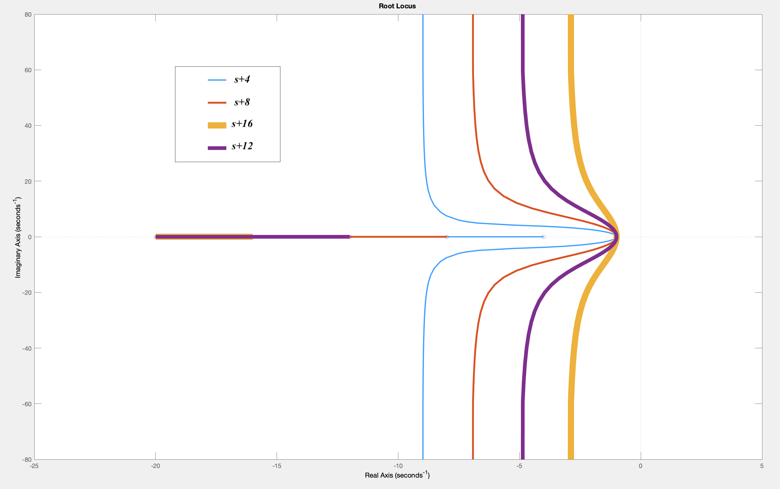
Root locus plots can be used to select a good controller. For example, for third-order system given by

H(s) = \frac{1}{(s+20)(s^2 + 2s+1},

we could use a controller with a single zero (or a proportional-derivative). To determine the best zero location, for example,

K(s) = (s+4), \;\;\; K(s) = (s+8), \;\;\;K(s) = (s+12),\;\;\; K(s) = (s+16),

we could use the following matlab commands to plot root loci for each of the controllers.

rlocus((s+4)/((s+20)*(s*s+2*s+1)))
hold on
rlocus((s+8)/((s+20)*(s*s+2*s+1)))
rlocus((s+12)/((s+20)*(s*s+2*s+1)))
rlocus((s+16)/((s+20)*(s*s+2*s+1)))

The above commands will generate a plot like the following (where we have recolored the lines and added a legend). Note that the controllers zeros at -4,-8,-12, and -16 generate root loci that have progressively less negative real parts, for worsening stability.

To plot the step response of the feedback system,

step(G)

The frequency response also shows the impact of including the first-order system in a closed loop, as can be seen in the plot generated by

bode(G)

For our third-order example, the step responses for the closed-loop systems can be compared, where notice that we have set a scale factor for each controller so that they all have the same steady-state value, K(j\omega)H(j\omega) for \omega = 0.

step(feedback((240*(s+4)/((s+20)*(s*s+2*s+1))),1))
hold on
step(feedback((120*(s+8)/((s+20)*(s*s+2*s+1))),1))
step(feedback((80*(s+12)/((s+20)*(s*s+2*s+1))),1))
step(feedback((60*(s+16)/((s+20)*(s*s+2*s+1))),1))

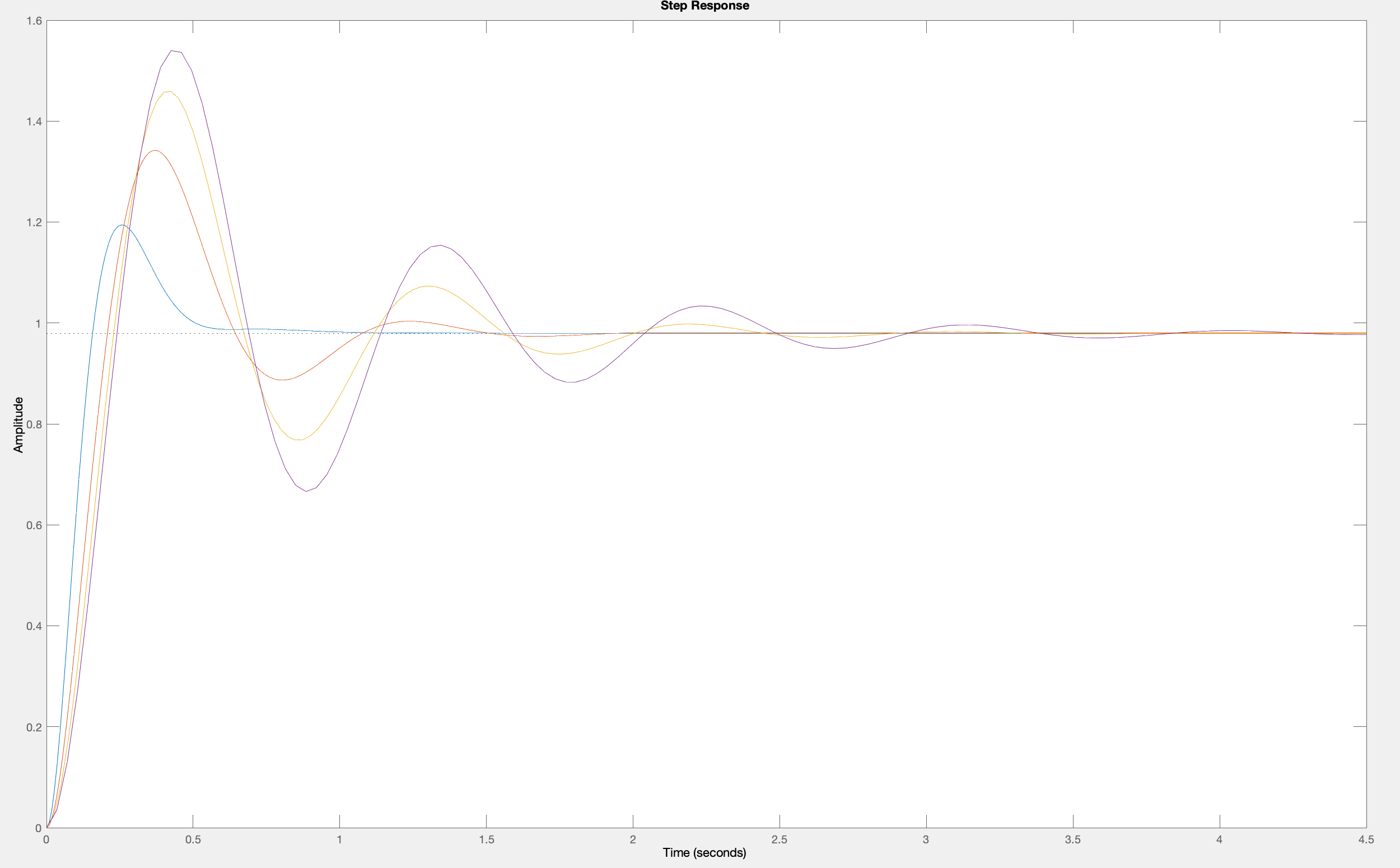
In the above plot, the step response for the s+4 controller has the smallest overshoot, unsurprising given the root locus plot. And what about the closed loop frequency response?

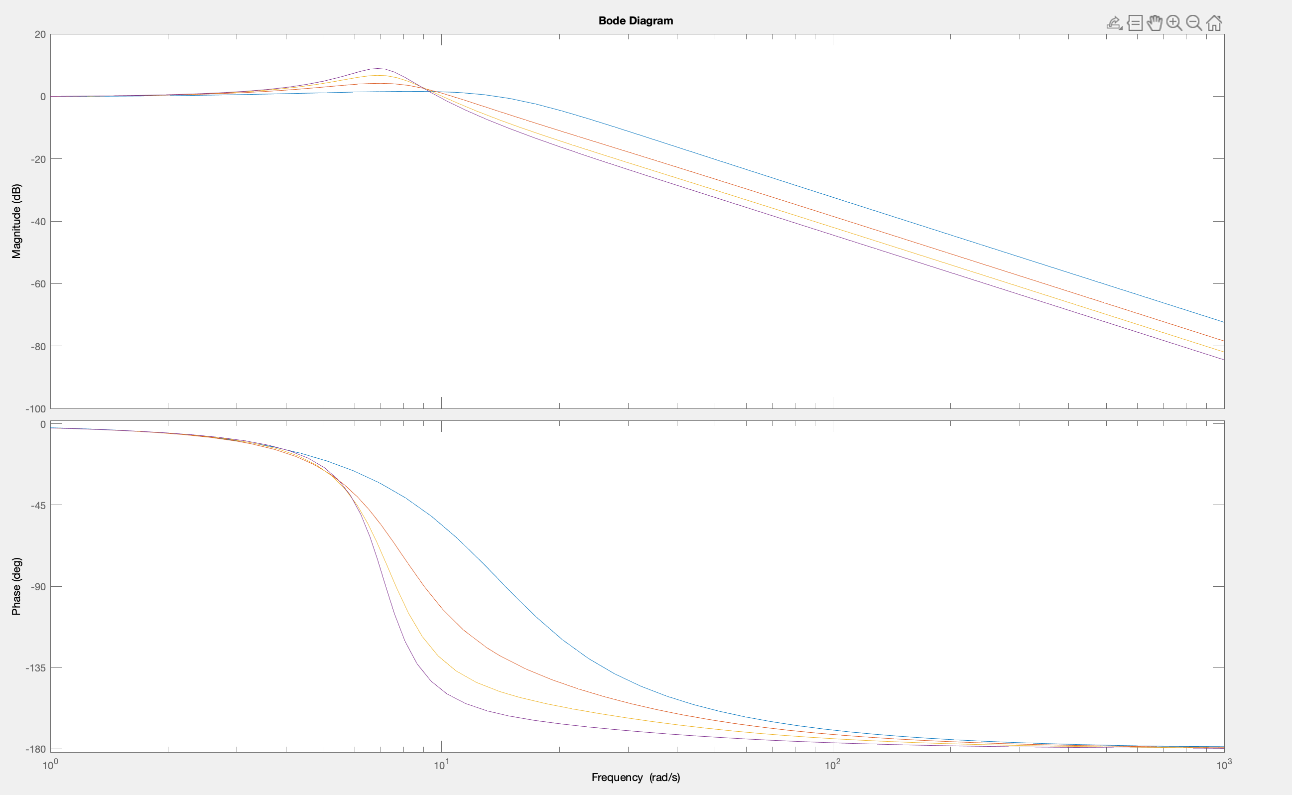
bode(feedback((240*(s+4)/((s+20)*(s*s+2*s+1))),1))
hold on
bode(feedback((120*(s+8)/((s+20)*(s*s+2*s+1))),1))
bode(feedback((80*(s+12)/((s+20)*(s*s+2*s+1))),1))
bode(feedback((60*(s+16)/((s+20)*(s*s+2*s+1))),1))

And the phase margin

margin(240*(s+4)/((s+20)*(s*s+2*s+1)))
hold on
margin(120*(s+8)/((s+20)*(s*s+2*s+1)))
margin(80*(s+12)/((s+20)*(s*s+2*s+1)))
margin(60*(s+16)/((s+20)*(s*s+2*s+1)))

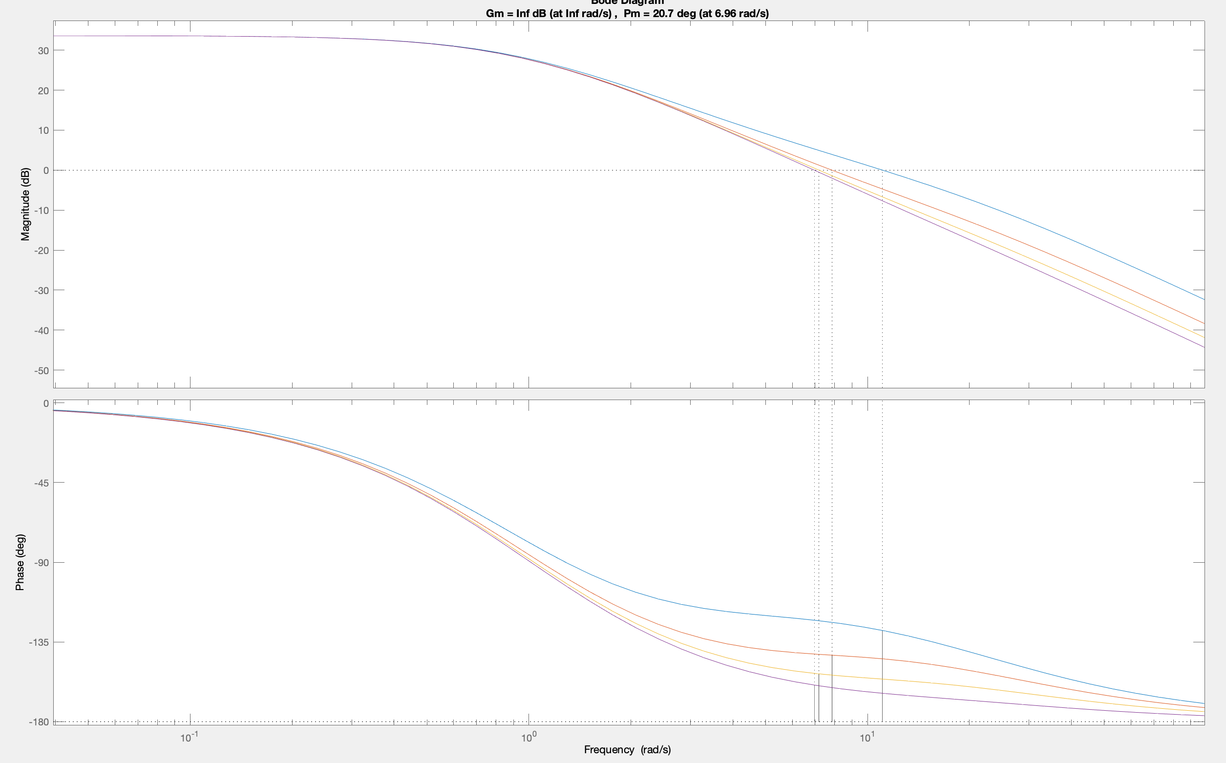
Notice that the s+16 controller resulted in a system whose step response had the most overshoot, whose frequency response had the most peaking, and whose phase margin was the smallest. Step response, closed-loop frequency response, and phase margin, they all they all tell the same story. The s+4 controller is more stable.

Now try yourself!

No such prelab: bode_poles_zeros
No such prelab: bode_steps
No such prelab: phasemargin