Win, Place, LQR
Please Log In for full access to the web site.
Note that this link will take you to an external site (https://shimmer.mit.edu) to authenticate, and then you will be redirected back to this page.
Quick Reference
NOTE: In the previous Maglev lab and in the Assembly guide, please note that the serial plotter is showing plots of 10 D_m , and ask you to calibrate the distance sensor to give values of 10D_m=-15,000 when the umbrella is right up agains the sensor, 0 when the umbrella is one black spacer away, and -15,000 when the umbrella is two spacers away. In this lab, we are plotting the distance, NOT TEN TIMES THE DISTANCE (sorry for this confusing change). For this lab, please calibrate the sensor to read DY_m = 1500 when the umbrella is right next to the sensor, DY_m= 0 when the umbrella is one spacer away, and DY_m=-1500 when the umbrella is two spacers away. Reasonable values for SensorScale should be between 0.2 and 0.4 and reasonable values for SensorOffset are between -1.0 and -2.5.
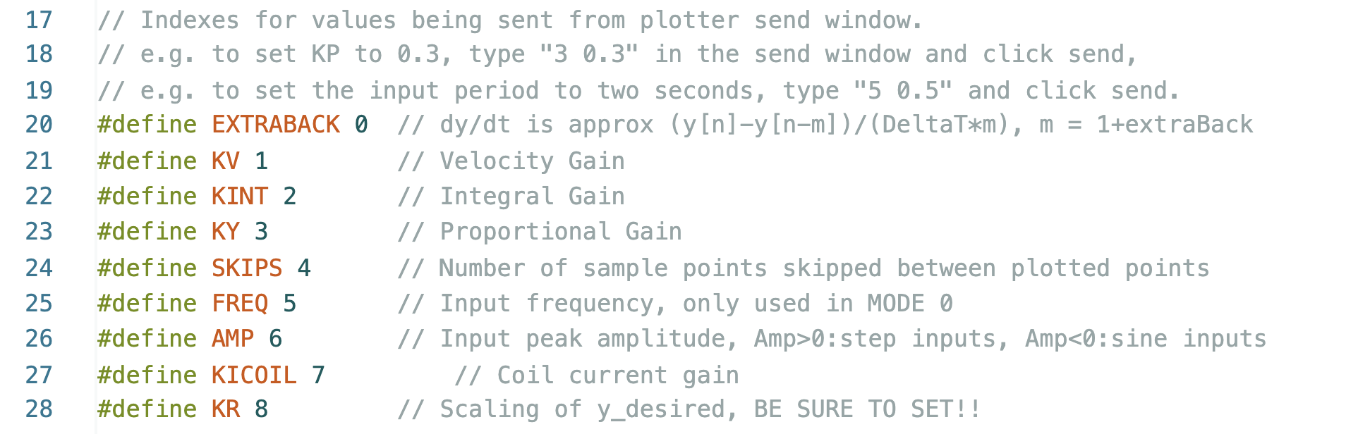
Serial Plotter Send Window Indices
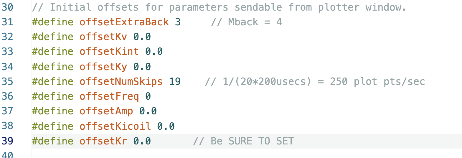
Useful Offsets to Set
Links
- Sketch for this lab (UPDATED FOR SS LAB!!) is here.
- Matlab script for this lab is here.
- We've created a "live script" version of the above matlab script. Outputs from live scripts appear in an adjacent window that one can scroll through (a little like the jupiter notebook environment for python). The live script version of the above sketch is here. Note: some of 6.310 staff love live scripts, others hate them. You should decide for yourself.
Task Summary
- Download this lab's Teensy sketch and the matlab code from the top of this lab, recheck that the electro-magnet coils are aligned, and that your values for SensorOffset and SensorScale still work (LOOK AT NOTE AT TOP OF LAB!).
- Determine and test a state-space model for the maglev system (Checkoff 1).
- Download the matlab script, fix all the FIX THIS FIRST issues.
- Fill in the A, B, and C matrices for your state-space model.
- Set the K and K_r values to implement a PD-like controller in both matlab and on the Teensy sketch.
- Verify that the matlab simulation matches your measured responses
- Fix all the FIX THIS SECOND issues in the matlab script, then try compute the feedback gains that optimize the matlab-simulated step response. Try using both pole placement and LQR weight selection to determine the gains.
- Test your optimized controller on the maglev system, and assess tracking and disturbance rejection (Checkoff 2).
- Add the integral term to the matlab state-space model, recalculate gains (including an integral gain) using LQR.
- Update the Teensy sketch and reupload. Assess the impact of including integral feedback on tracking and disturbance rejection (Checkoff 3).
In this lab, you will be designing state-space controllers for your Maglev system, but you will not be starting over, as we hope to make clear in this section.
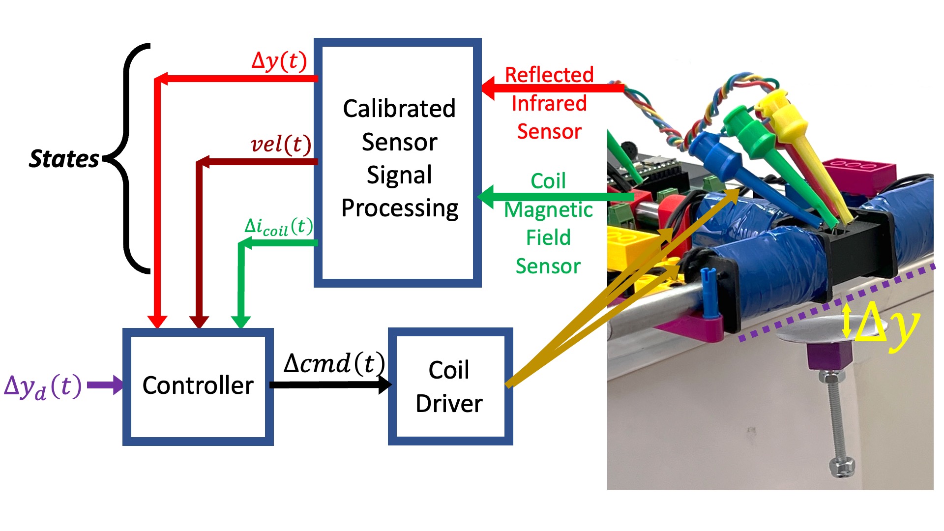
In order to design a better-than-PD controller for our maglev system, we needed an accurate model. We used a combination of analysis and measurement to determine a transfer function model for the system, or more specifically, for the green encapsulated region in the maglev system diagram below.
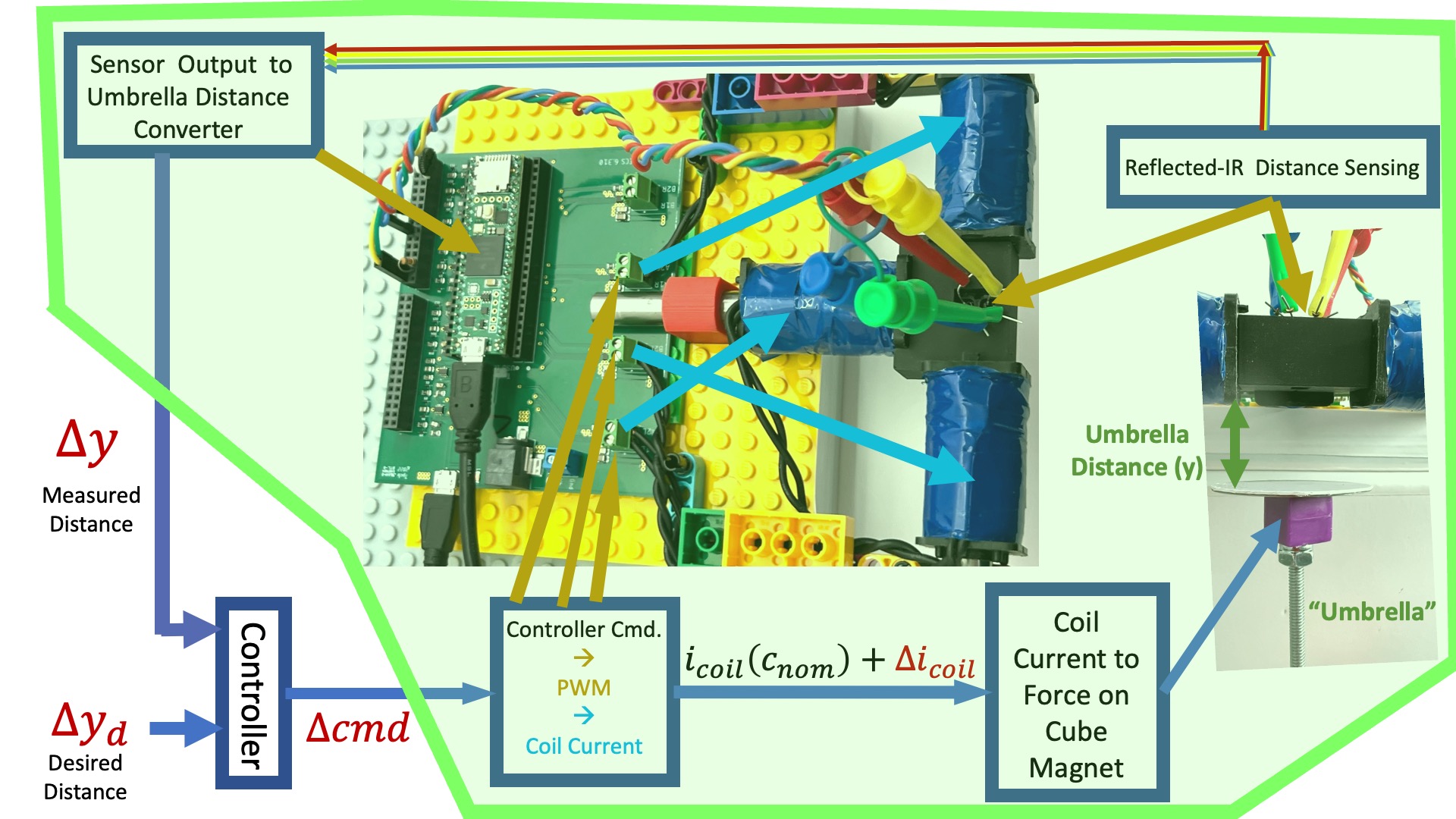
As the green encapsulated region in the above figure makes clear, our maglev model had a single input, the change in micro-controller command (\Delta cmd), and a single output, the measured change in umbrella position (\Delta y).
The single-input single-output maglev transfer-function model is shown in the block diagram below (and labeled H_{c2y}(s)), where it is combined with a "lead" controller, labeled K(s), and embedded in an umbrella-position-controlling feedback system.
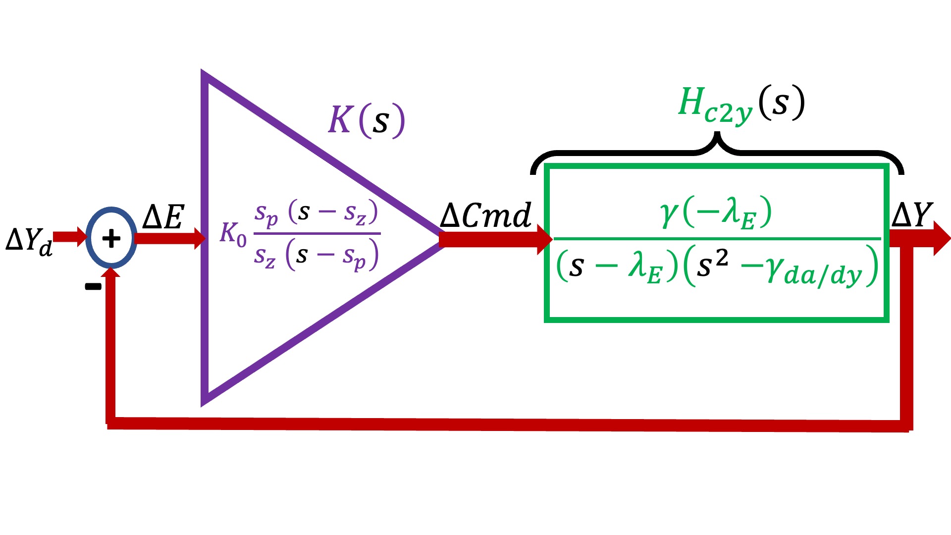
In the above block diagram, the maglev model (in green and labeled H_{c2y}(s)) has three model parameters, \gamma, \lambda_E, and \gamma_{\frac{da}{dy}}, and the lead controller (in purple and labeled K(s)), has three design parameters, s_z, s_p, and K_0. In the last lab, we used a variety of measurements to determine H_{c2y}(s)'s model parameters, and then used that calibrated model (along with the concept of phase margin) to determine K(s)'s design parameters.
We are using an optical sensor to estimate umbrella position, are using its sample-to-sample variation to estimate time derivatives, and are using a magnetic field sensor to estimate coil currents. Effectively, we are measuring the umbrella's state: its position, its velocity, and its acceleration (coil current is proportional to force, force is proportional to acceleration). Yet we are not using state-space control, we are not even using all the states we can measure. Coil current is ignored by our PD and lead controllers, its measurements are only being used for model calibration.
As an alternative, consider the system diagrammed below, in which the controller uses measurements of coil current, umbrella velocity and umbrella position to determine command updates to the coil driver.
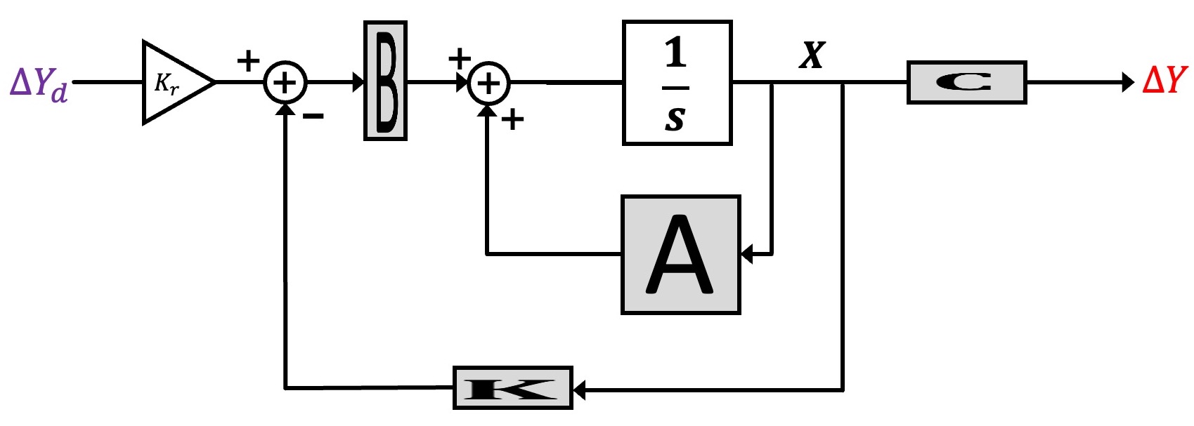
We could then use a linear state-space controller, like in the figure below.
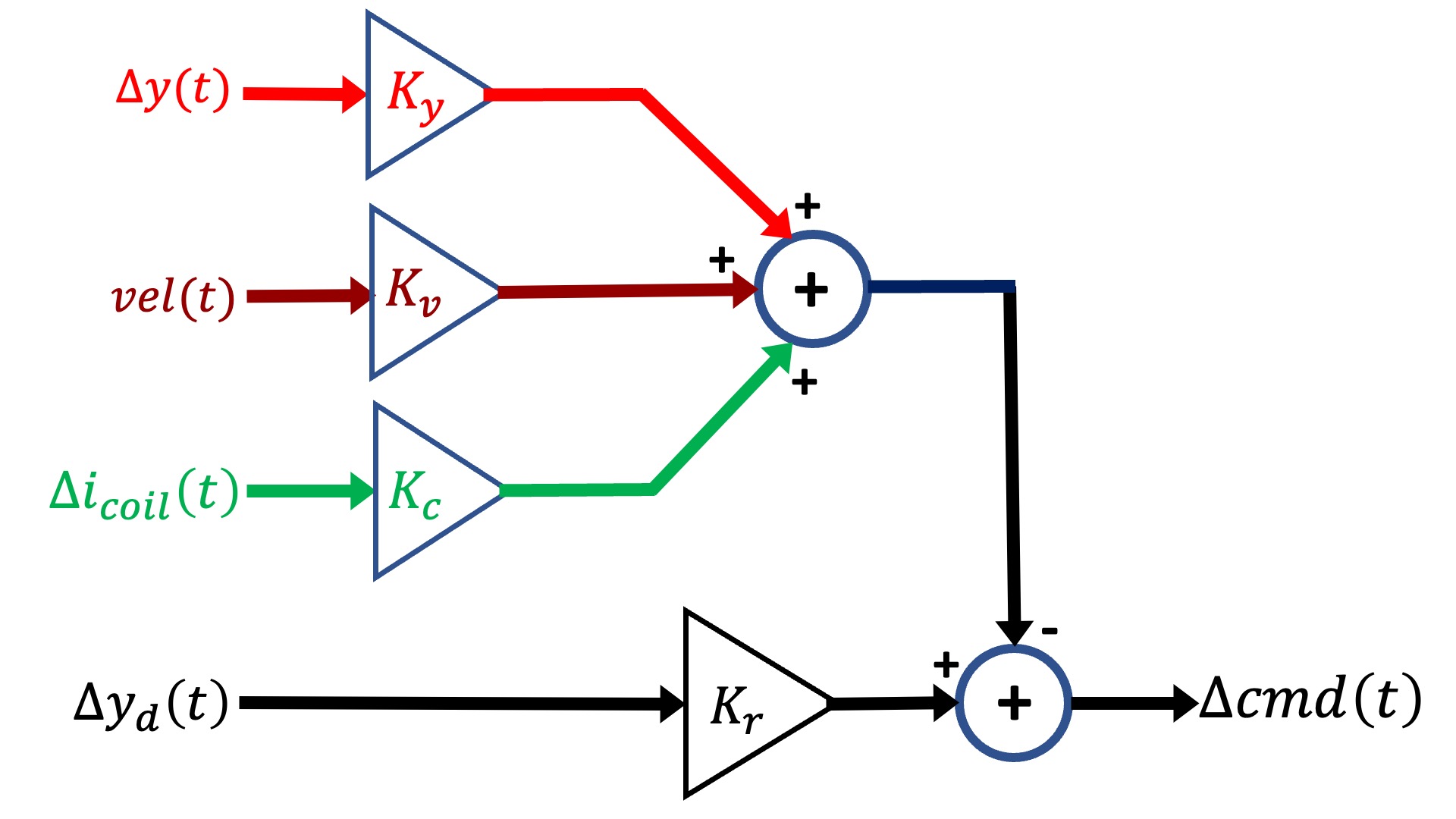
It was difficult enough to design the lead controller when we only had three parameters to determine, s_z, s_p, and K_0. And as the above diagram makes clear, we now have four, the three state "gains", K_y, K_v, K_c, and the input scaling, K_r. There are computational tools that will help us find reasonable values for the K's, given a state-space model for our system.
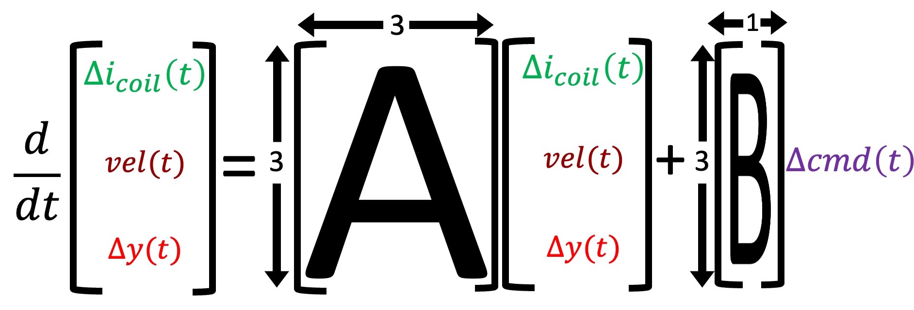
Consider the state-space model differential equation,
We summarize system with the states and matrices below.
In standard state-space feedback, u(t) = \Delta cmd(t) is given by a scaling of a desired input, K_r \Delta y_d(t), minus feedback from a weighted combination of the states, -K x(t), as shown in the block diagram below.
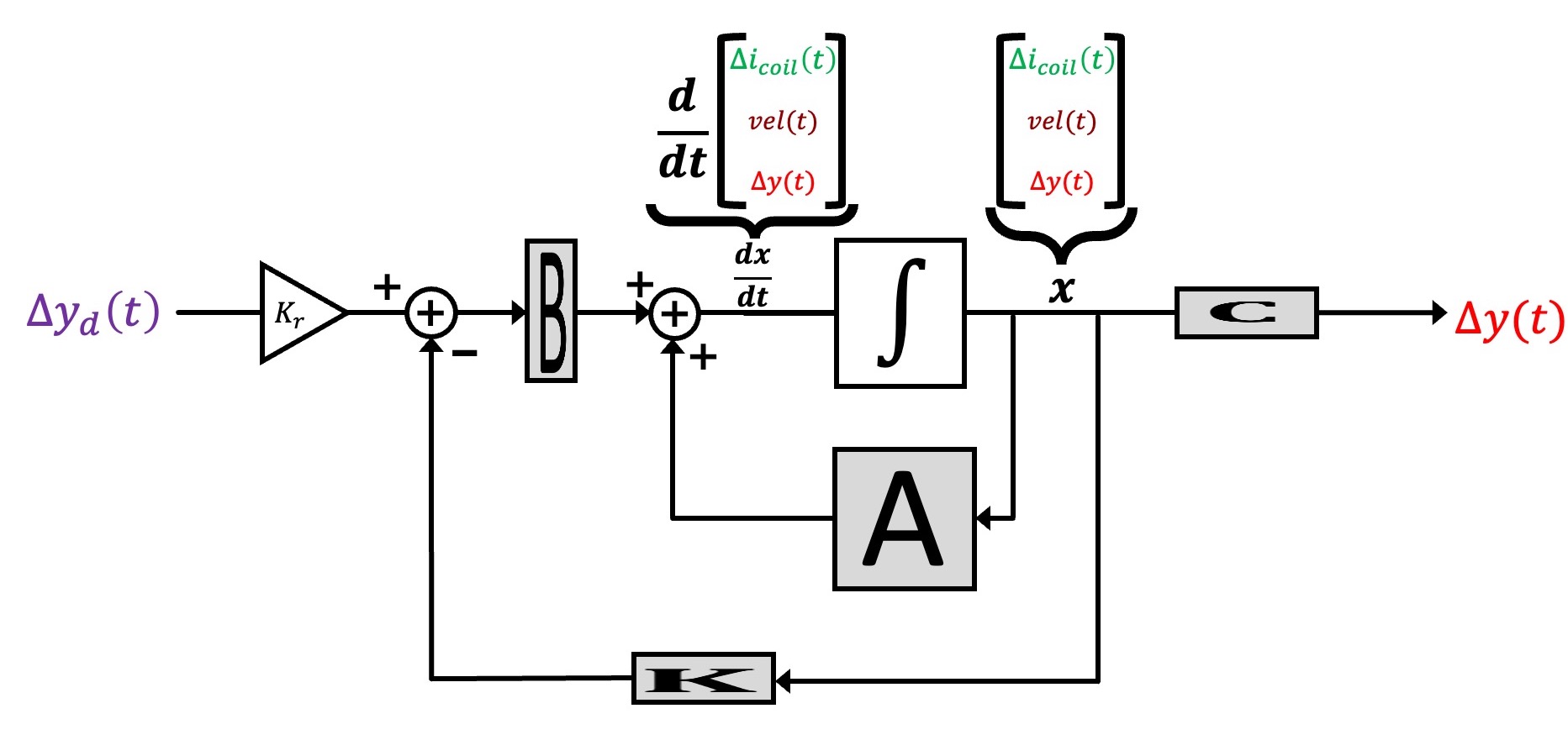
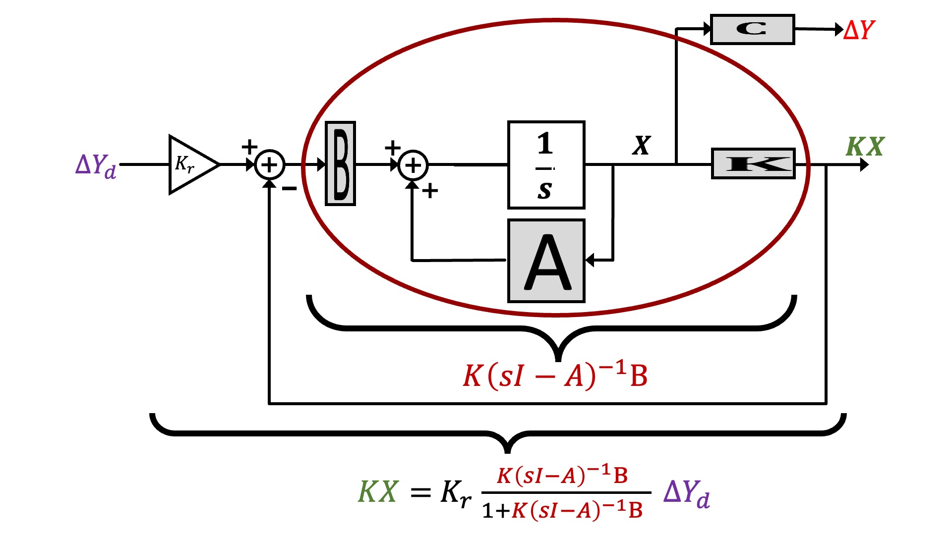
We can represent the block diagram in transfer function form, as shown below.
And finally, we can reorganize the state-space description to make its description look more like the feedback loops we have been analyzing with Black's formula, as shown below.
Fortunately, in the last lab we created and carefully-calibrated a model of our maglev system, but unfortunately, the model is in transfer-function rather than state-space form. And transforming the transfer-function model to a state-space model requires that we pick states consistent with our measurements. Tackling this problem will be this lab's first challenge.
With our carefully-calibrated transfer function model for our maglev system, H_{c2y}(s), we can generate the state-space model using one of the many automatic procedures for converting transfer functions into state-space models (e.g., controllable canonical, observable canonical, modal, etc). That there are so many conversion algorithms hints at a key issue: while there is only one transfer function associated with a given \{A,B,C,D\} state-space model, there can be an infinite number of state-space models that generate a given transfer function, and an associated infinity in the choice of state variables.
What we need is a state-space model whose states are consistent with our measurement of umbrella position, umbrella velocity, and coil current. That is, we must find an \{A,B,C,D\} state-space model for our maglev system that satisfies two criteria:
- its states are umbrella position, umbrella velocity, and coil current;
- its transfer function matches the our carefully-calibrated maglev transfer function.
To start the process of mapping the transfer function into the A and B matrices in the above figure, consider unraveling the H_{c2y}(s) transfer function back into a product of two transfer functions, one from Teensy command to coil current and one from coil current to umbrella position as shown below.
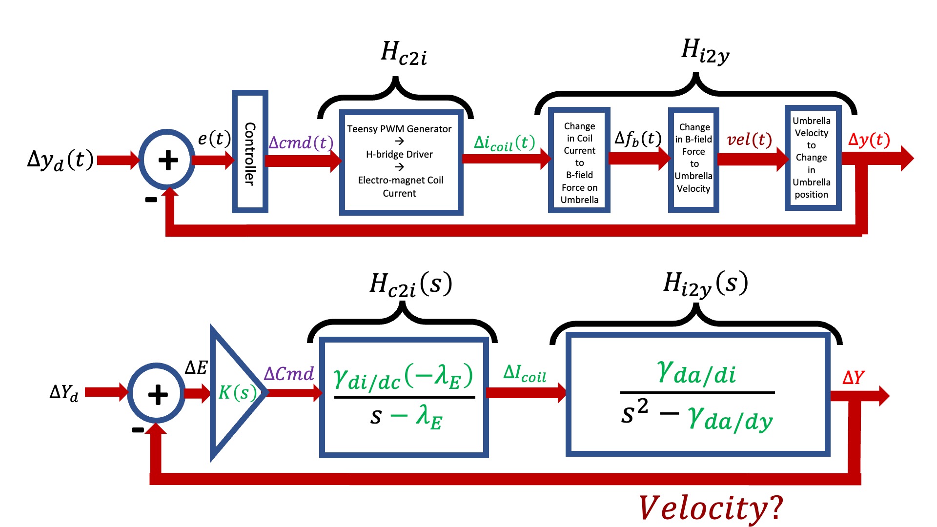
As noted in the above figure, we now have an explicit \Delta I_{coil} and an explicit \Delta Y that correspond to the first and third states, but we do not have anything explicit relating to velocity. Nevertheless, from H_{c2i}(s) we can determine the differential equation that relates Teensy command to coil current, and map its coefficients into the appropriate matrix elements in the first row of A andB, as shown in the figure below.
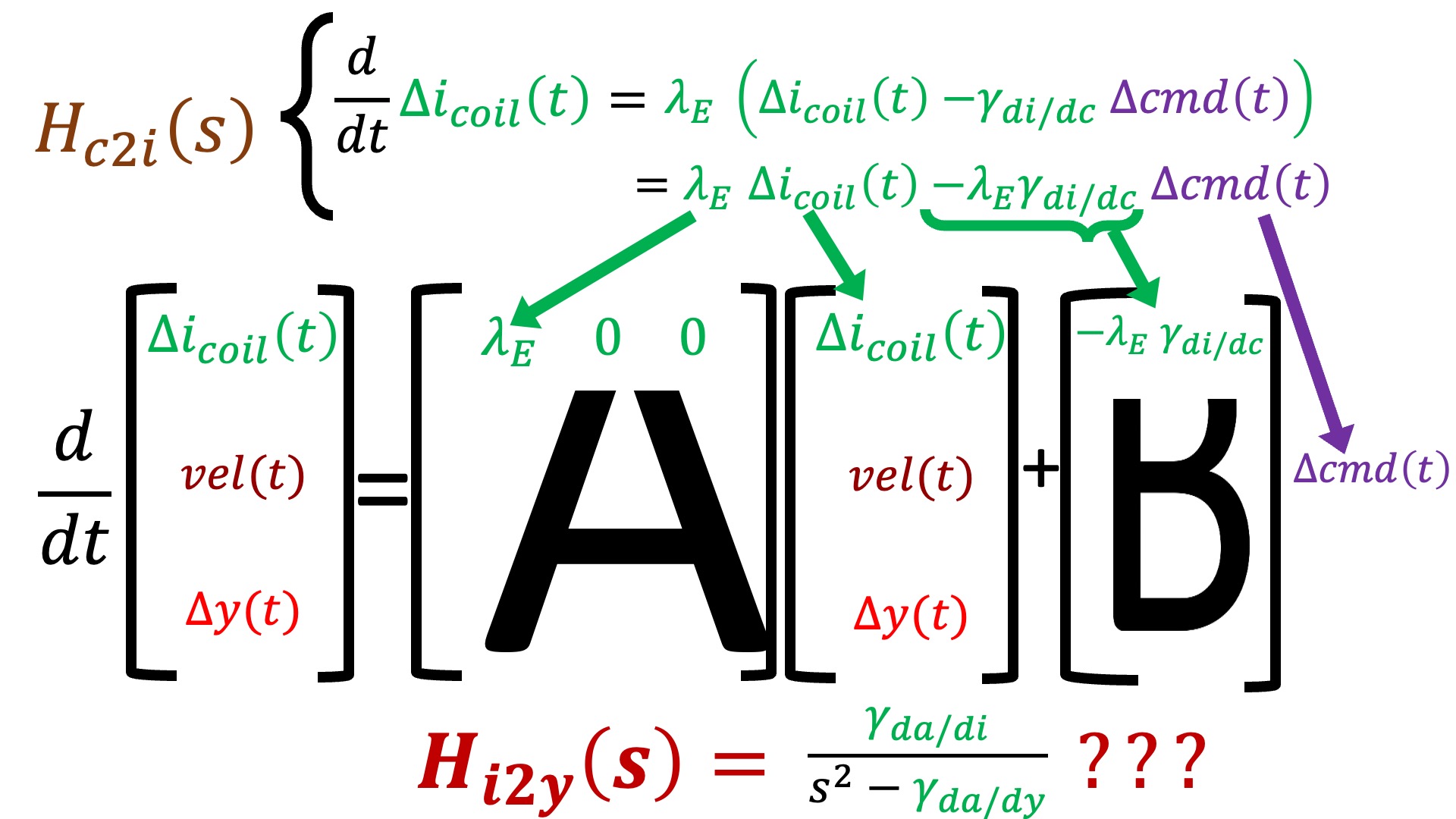
In the above two figures, we noted that velocity is missing in the transfer function and H_{i2y}(s) is unused in constructing the state-space model. And, of course, the bottom two-thirds of A and B are unspecified.
We have provided a matlab script with the structure of a state-space model for maglev. If you examine the script (and try running it), you can see that we left out more than just the model. (calculating closed-loop matrices, K_r, etc). Look for lines with FIX THIS FIRST!!!* and fix them.
Note that we created a system with multiple outputs, defined by the matrix Cplot in the matlab script. We did this so that when we used matlab's step command, plots of all three states are generated, not just position. But we also want to plot one more quantity. Recall that u = K_r y_d - K x, and that in our case, u = \Delta cmd, and its plot should not exceed 10 by much, or be much smaller than -10 (\Delta cmd will saturate the coil driver if outside the range -1 to 1, and we scale that by 10 because matlab is simulating a unit step, and we typically take steps of 0.1). The step function will plot u = K_r y_d-K x if we prepending a row to the Cplot matrix and add a single non-zero value to a 4 \times 1 Dplot matrix.
For state-space models, D is used to represent a direct contribution of system's input to its output, as in
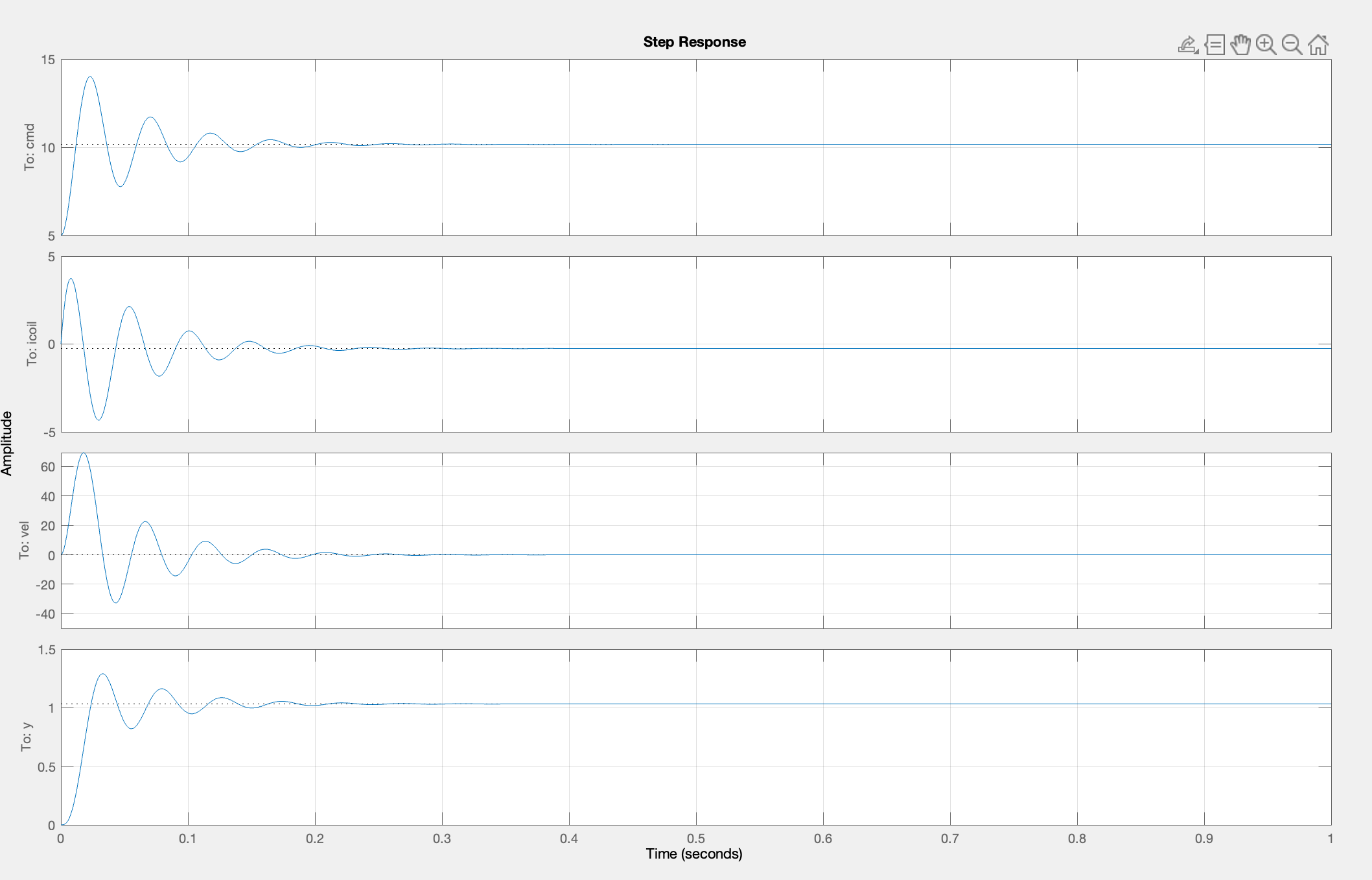
Please use your insight into state-space modeling, along with the hints above, to find and fix all the FIX THIS FIRST sections of the matlab script linked at the top of this page. If you have implemented a reasonable state-space model, and have set values for K and K_r that produced oscillations with your PD maglev controller (lines 97-99 in the matlab script), and fixed all the other FIX THIS FIRST issues, the script should produce two figures (often right on top of each other). Uncover figure one, it should look something like the image below. The script is simulating the behavior of its model of the maglev arm system (using the PD controller you should have specified), and plotting the results. You should see four plots, and from top to bottom they are: the Teensy command being sent to the maglev coil drivers, i_{coil}, vel and y.
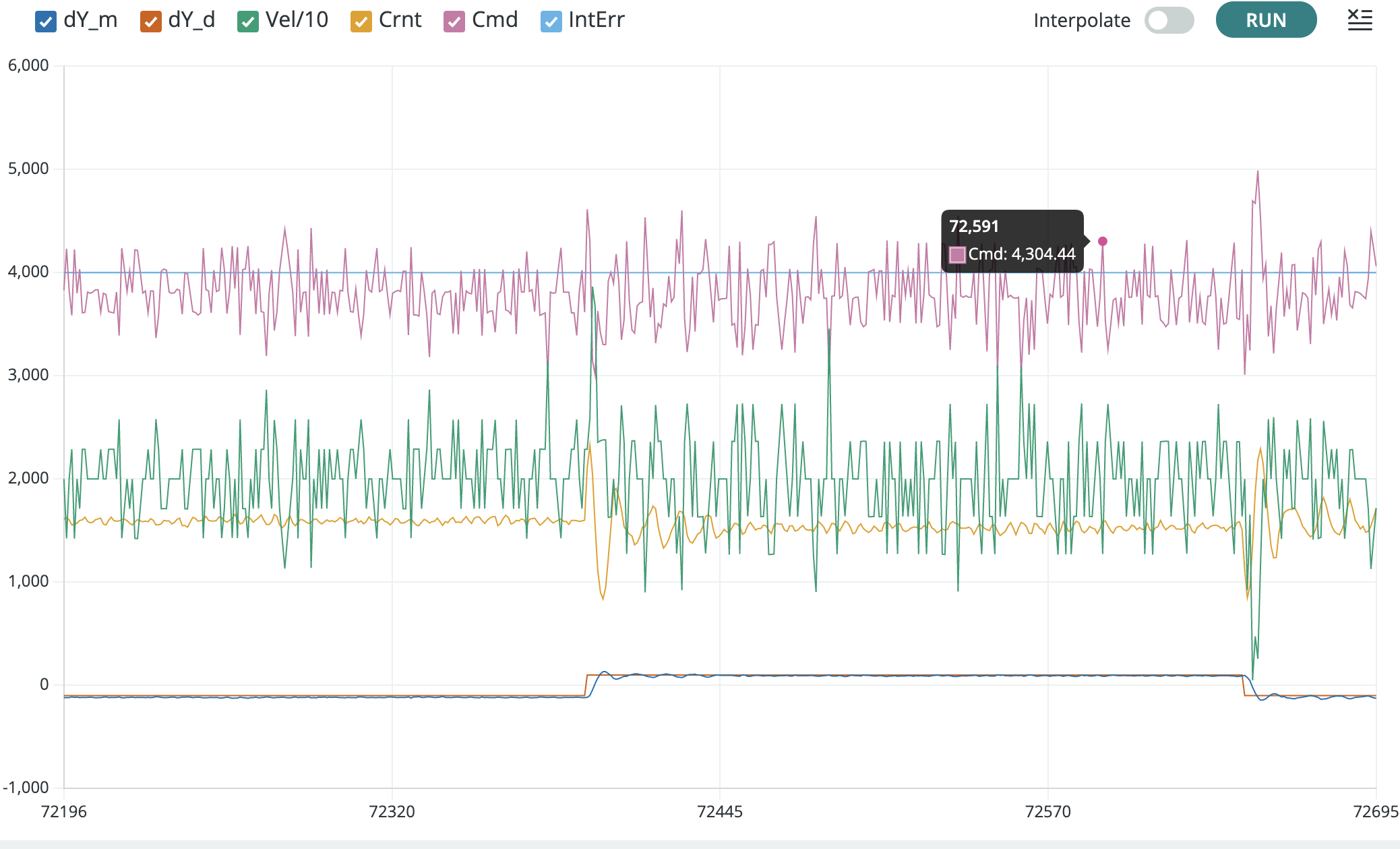
Once you have the matlab script producing reasonable outputs, plug in both power supplies, upload the 6310_MAGLEV_SP23_SS Teensy sketch (linked above), and start the serial plotter. When you start the serial plotter, you should see a plot of six waveforms (this time starting from the bottom and working up): \Delta y, the umbrella position (in the last lab we plotted 10x this value); \Delta y_d, the desired position (in the last lab we plotted 10x this value); vel/10, the umbrella velocity scaled by 10 (in the last lab we plotted 10x this value); Crnt, the electromagnetic coil current; Cmd, the Teensy command to the coil driver; and intErr, the integral of the position error. A typical plot snapshot is shown in the figure below.
Use the plots and your umbrella to check that your distance sensor is still calibrated, but PLEASE SEE THE NOTE AT TOP OF THIS LAB (THE DISTANCE PLOT IS NOT SCALED BY 10 UNLIKE THE LAST LAB AND THE ASSEMBLY GUIDE. IF YOU DETERMINE VALUES FOR SENSOROFFSET AND SENSORSCALE THAT ARE VERY DIFFERENT FROM THE VALUES YOU USED IN THE LAST LAB, SOMETHING IS WRONG, ASK FOR HELP). Once you have checked the distance sensor, use a compass to check that the coil directions for the electromagnet are still consistent.
After you have checked the sensor and the coils, use the Teensy sketch offset definitions (lines 31 to 39) to set values for the K's that implement your PD controller (and maybe set the amplitude of the desired value to 0.1 and its frequency to 0.5, though you can also do that from the send window when running the serial plotter). Then refloat your umbrella (you may need to adjust the potentiometer, just like last lab).
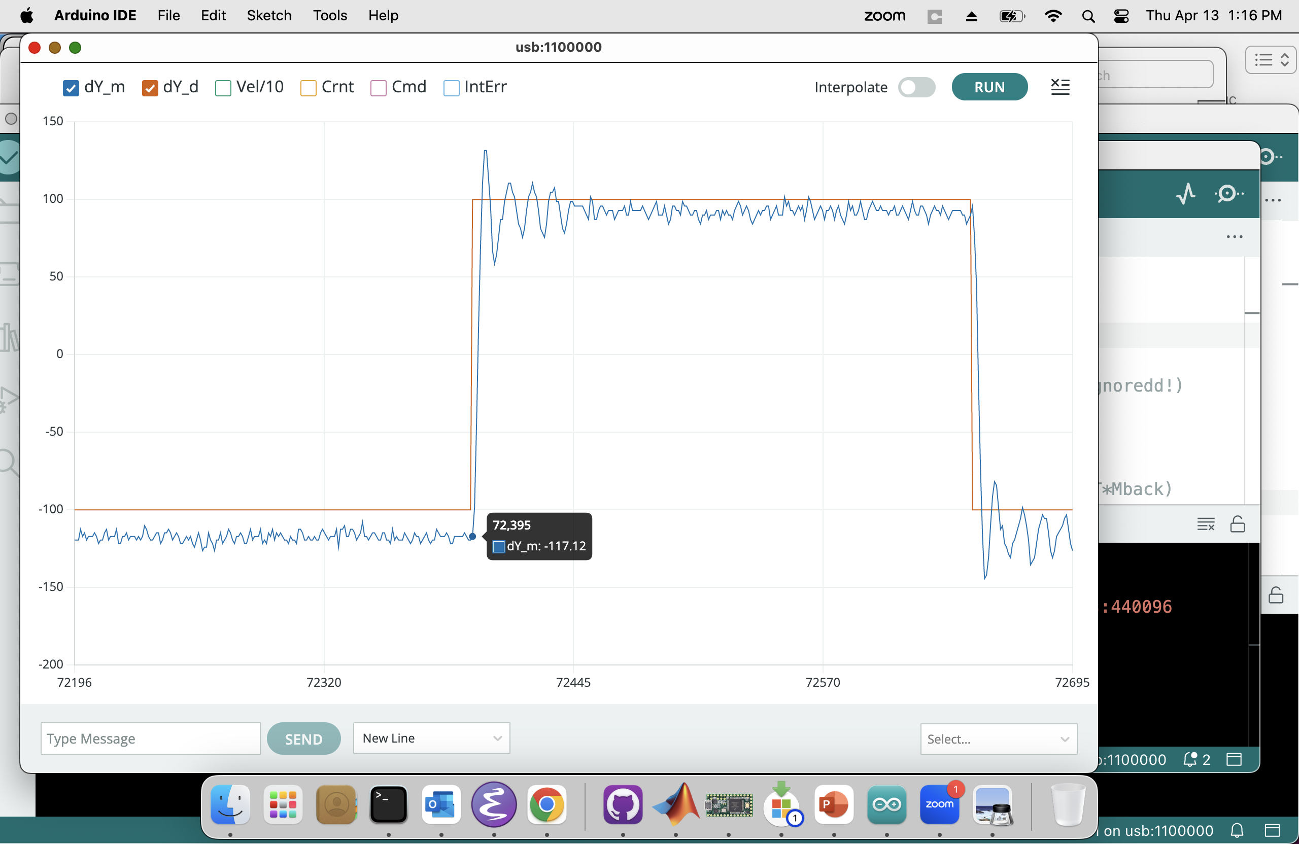
You can unclick all but the \Delta y and \Delta y_d, to focus in on the position errors, as shown below.
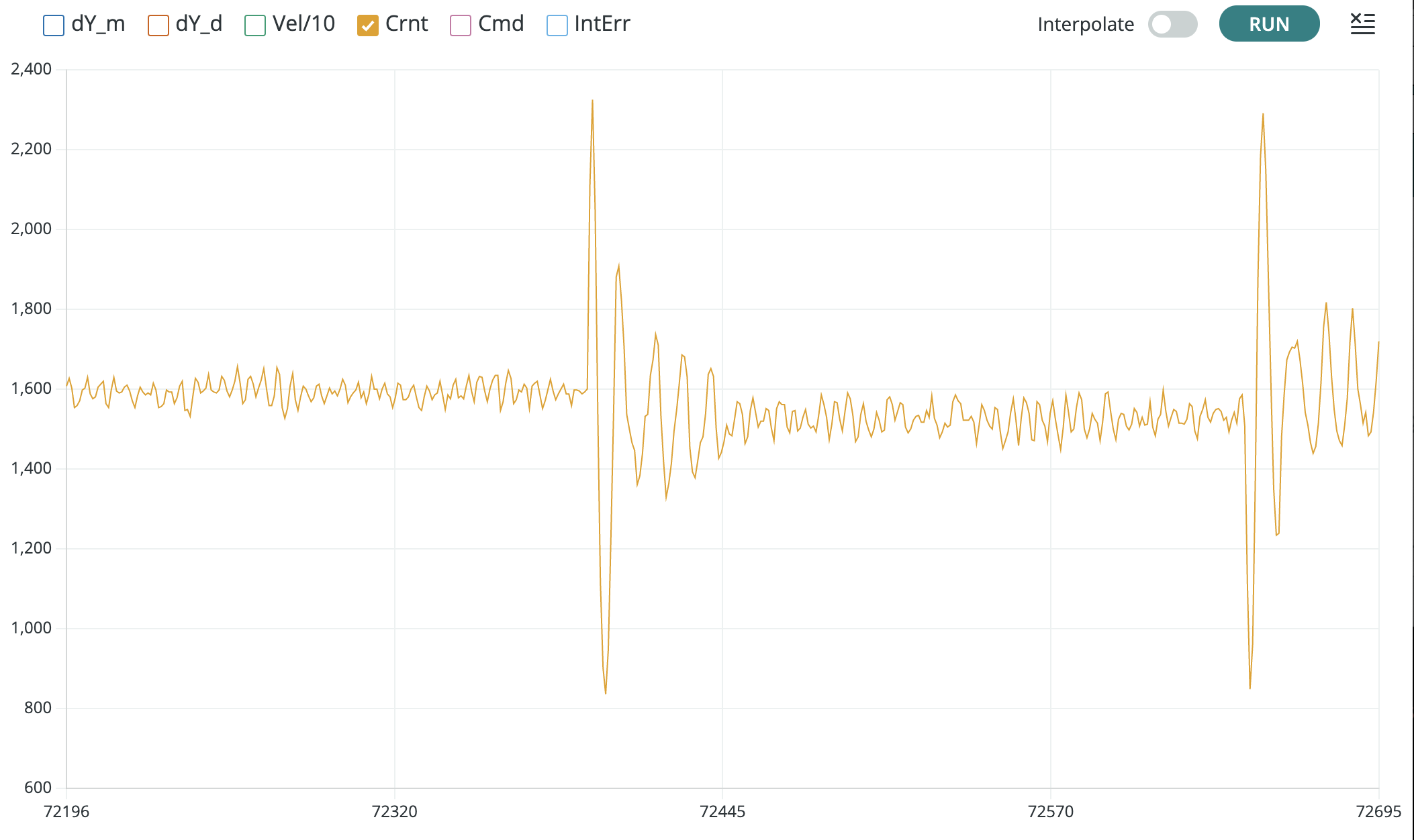
Or unclick all but the Crnt to focus in on the coil current scaling, as shown below.
You should be able to compare the plots from the Teensy serial plotter to the simulation outputs from matlab. If your model is a good match, then you should see results like the ones shown in the figures below. If model and simulation are mismatched, tweak the model parameters until you get a good match. The better your model, the better the resulting controller.
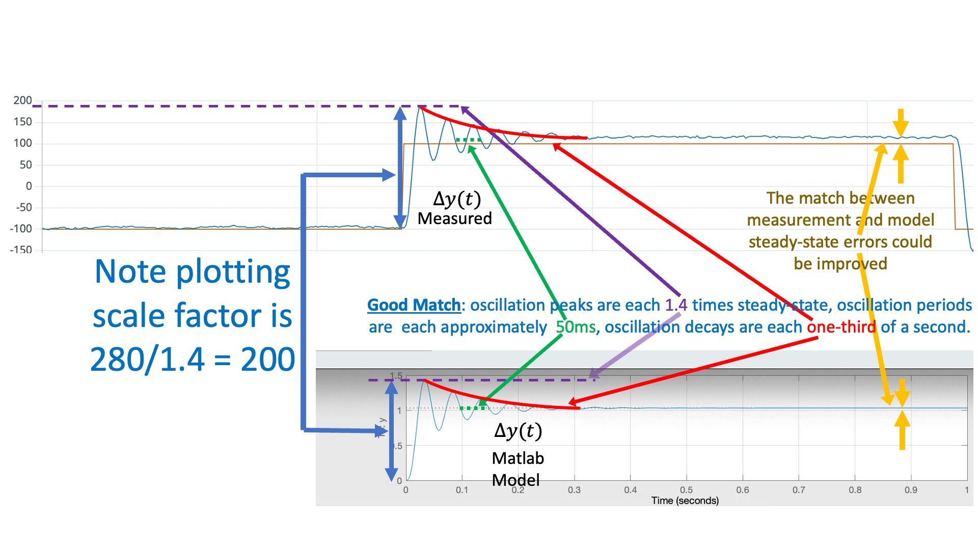
In the figure above, we compare the simulated and measured umbrella position, to check that they have the same "shape" (initial overshoot, oscillation period, oscillation decay time). Note that there is a scale factor between the plots that reflects a scale factor in step size. Matlab is using a "unit step", but when we set the square wave amplitude to 0.1 in the Teensy sketch, we can see (from the red y_d plot) that we generate a step of 200 (-100 to +100) in the units of the serial plotter. So the measured step is 200 times larger than the matlab simulation (again in the plotting units).
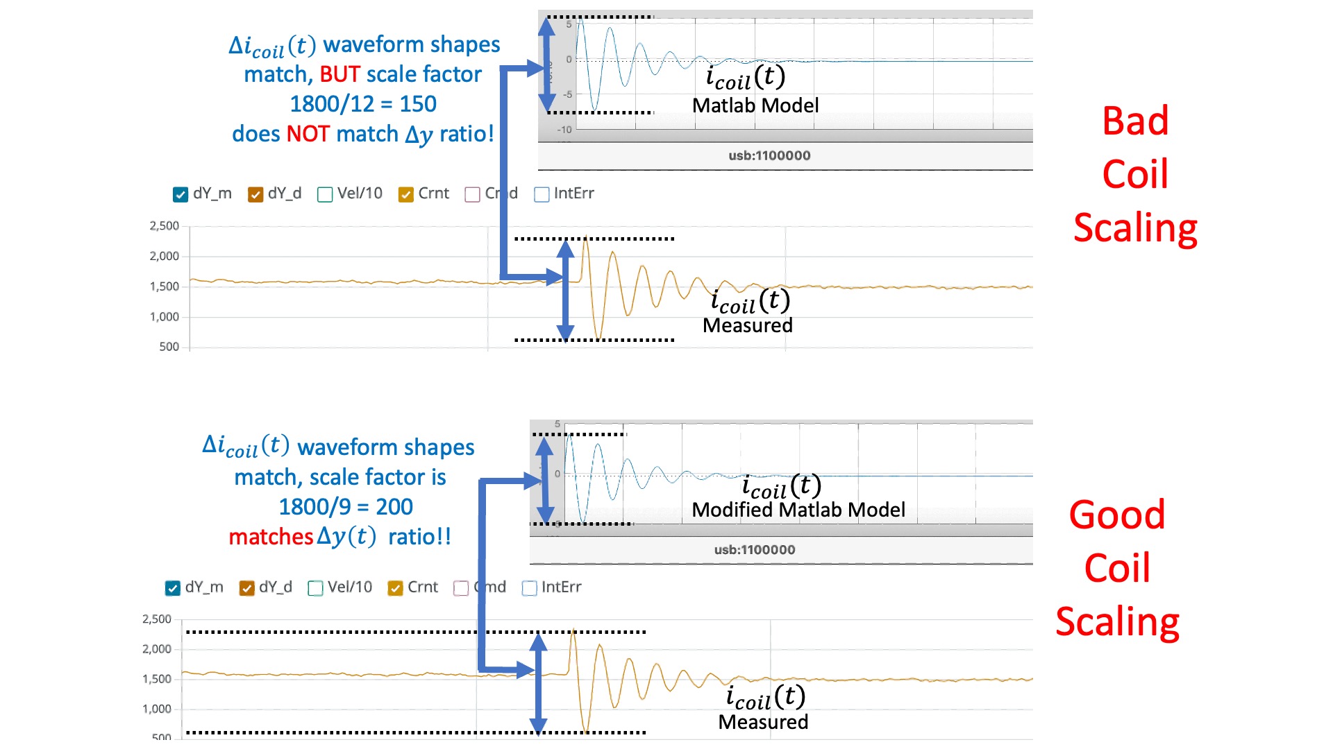
When comparing coil currents, as in the figure below, there should be the same scale factor of 200. So the measured current should have the same shape as the matlab simulation, and should be 200 times larger.
Mismatched scale factors between measurement and model are BAAADDDD! If the scaling is not consistent in the model, then when you use that model to compute state feedback gains, those gains will be incorrectly scaled. And with incorrectly scaled gains, chances are your feedback system will be UNSTABLE!

The first time we used PD control, we eyeballed gains or used models to do the search and then tweaked the gains after examining the results. Now we are going to use a "somewhat" more systematic way of picking the gains, either by selecting a desired set of closed-loop poles and computing the needed gains, or by adjusting state and inputs weights and then computing the cost-minimizing gains.
When experimenting with picking poles or weights, you should be iterating. That is, pick a set of poles or weights, determine the K's, run the simulation, and if you like the simulation, try the gains on the maglev system. If you don't like the maglev performance, try to adjust the poles or weights to improve performance and repeat the above process. NOW HERE IS THE IMPORTANT POINT! If you are unhappy with the performance of a controller designed by placing poles, it can be very difficult to determine how to rearrange those poles to improve performance. But if you are unhappy with the performance of controller designed by choosing LQR weights, you can probably determine how to adjust the weights to improve performance. But this you should experience for yourself.
With full-state feedback, we can have a dramatic effect on the eigenvalues of the open-loop \textbf{A}. That is, given certain conditions (which are met in this case), we can adjust the gains to place the eigenvalues of the closed-loop \textbf{A}_{cl} anywhere we want. That is, by picking \textbf{K}, we can move
For a simple second order system like you saw in the prelab, you can very easily solve "on paper" for gains given a desired eigenvalue placement. For larger systems, beyond third order, there is no closed form for the eigenvalues, and finding the gains for a given placement is best done computationally. We can rely on numerical approaches for determining K given \textbf{A} and \textbf{B}, such as Ackerman's method and its variants. Matlab's place command does exactly what we want, provided we do not try to place poles right on top of each other,
% A = your A matrix
% B = your B matrix
p = [-1 -1.23 -5.0]; % poles must be unique
K = place(A,B,p)
Unfortunately, even though we have a function that will take desired eigenvalues(aka poles) and return the needed gains, that does not mean we can just set the closed-loop eigenvalues to be real and put them at -\infty. If we could, then our system would respond infinitely quickly to changes in desired position, and who wouldn't want that?
What happens when we make the poles too negative? What physical limitations stop us from choosing arbitrarily negative poles?
We strongly recommend you review section 3.1 in the "State Space And LQR" question on the prelab here.
As you are setting weights, consider the relative magnitudes of the position, and the velocity. The umbrella does not move very far, but it can move very fast. What does that say about the relative weights for position and velocity?
You can use pole placement or LQR to design better controllers, and then simulate the results, once you have found and fixed the parts of the script labeled *****FIX THIS SECOND!!!****.
Be sure to comment out lines 97 and 98 in the matlab sketch (to remove your PD controller), and uncomment either line 87 (for LQR) or line 88 (For Pole Placement).
When transferring the K's you compute in the matlab script to the Teensy sketch, we STRONGLY recommend that you copy the gains from matlab to the offset values in the sketch (lines 32, 33, 34, 38 and 39), and then upload. Trying to set four values using four different indexes from the send window in the serial plotter is too error prone.
Below are some senarios to try when testing your controller. In particular, be sure to try adding weight to your umbrella, to test your controller's disturbance rejection.
Show your corrected matlab scripts and simulation results.
margin(ss(A,B,K,D)) (see the last figure in section 1.3 above).
STOP HERE FOR WEEK A!!!!
Fix the matlab script so that it will use LQR to calculate the gains for the maglev model plus and extra state, the integral of the error (once you have fixed FIX THIS THIRD!!!** sections). See the Prelab for more details about adding the integral term, and think carefully about what happens to K_r.
So how will you set the weight on the integral term? You want it to go to its steady-state value quickly, like all the other states, but is the integral the same scale as the other states? Suppose a sudden disturbance displaces the umbrella a tenth of a millimeter in a millisecond. The measured error in \Delta y will also change by 0.01 in that same millisecond, but what about the integral of the position error? An error of 0.01 would have to persist for a 1000 milliseconds before the integral of the errors rises to 0.01. What does that say about the relative weights for these two states?
Once you have fixed the matlab script, try computing state gains for all the states, including the integrator, using LQR. Once you have gains that result in good performance in simulation, test them on the maglev system (the integral gain is Kint, in the Teensy sketch, or index 2 in the send window). Below are some senarios to try, be sure to test your system's disturbance rejection using extra magnets.
Show your corrected matlab scripts and simulation results.