Observer and Learn

1) CHECK-OFF RULES!!!

For this final lab, the check off rules are a little different.

1.1) ALL CHECKOFFS ARE ONE-ON-ONE

You can work with a partner, you can solve the lab together, you can check off with shared hardware, but we would like to do this last lab's checkoffs one-on-one. The diversity of your linear algebra backgrounds is too great, and we want to make sure we have not left any of you with misconceptions. As always, the is NO penalty for repeats. So if you are not sure of what you are not sure of, let us help you figure it out.

2) Introduction

We will start this lab by repeating LQR control, but in discrete-time (so the states are measured, and feedback gains are determined using our model and DLQR, discrete-time LQR). Then we will avoid measuring states directly, and instead, estimate them using discrete-time state-space model simulation with angle measurement corrections.

We have done our best to help you avoid pitfalls. As you will see, we have made significant use of simulation in matlab, and to reduce frustration, we have streamlined the process of moving controllers from matlab to the Teensy. The use of matlab is easiest if you have a local installed copy on your computer. But since many of you have been using the online matlab, you can continue to use it (see the on-line matlab instructions below).

2.1) Task Overview.

In this lab you will return to the double-drive-propeller arm (with both propellers driven by parallel drivers, mostly eliminating the heating problem), but this time, you will use the simple PD controller to stabilize the arm, and then use its behavior to improve a continuous-time state-space (CTSS) model of the arm, which is converted numerically to a discrete-time state-space (DTSS) model. You will use this calibrated DTSS model, along with LQR, to select gains for a discrete-time measured-state feedback controller, and test candidate gain sets on your propeller-arm. As you will see, a key problem for measured-state feedback control is its sensitivity to noisy state measurements. This is an issue for our copter-arm system, since two of arm state measurements, rotational velocity and backEMF, are quite noisy.

Instead, we can estimate the hard-to-measure rotational velocity and backEmf states by using the DTSS model to simulate the copter-arm system, and correct the simulation using only the lower-noise measurements of arm angle. This continuously-corrected simulation, usually referred to as an "observer", introduces a new problem, selecting correction gains. Selecting the gains involves a trade-off between fast estimate convergence and noise magnification, as you will see.

In an observer-based controller, the controller must perform simulation, so it needs a copy of the DTSS model (the \textbf{A}_d, \textbf{B}_d, and \textbf{C}_d matrices), as well as the state-feedback and observer gains (K_d and L_d). Even for a three-state system like ours, that is too much to copy over by hand. Instead, we are providing you with a matlab script, propSS.m, that automates the process of generating the DTSS model and controller gains, and transferring it to a Teensy sketch, 6302_Obs_Fall21. The propSS.m script calls the function propModel to generate the CTSS model, converts the CTSS model to a DTSS model, calls function dtObs.m to design the controller and observer gains, then calls the function DTSim to simulate the system and controller, and finally calls the function printTeensyObserver to generate the include file for the Teensy sketch. If you examine the functions, each in their own file, you will see that many are "unfinished". You can finish them by searching for FIX THIS.

The two propeller system with an observer-based controller can be quite impressive, and you should be able to do better than this video of the observer-based controller in action. Notice how badly it overshoots on the very large steps, but it is rotating nearly 300 degrees.

2.2) Key Concepts

There are a number of key ideas in this lab, including:

• A good strategy for designing controllers is to use a simple controller to stabilize a system, so that you can take measurements and calibrate a state-space model, and then use the state-space model to design a more sophisticated controller.
• State-space models for physical systems are usually easiest to write down in continuous time, but conversion from continuous time (CT) to discrete time (DT) is a necessary step if one is designing an observer-based controller.
• In state-space, conversion from CT to DT is automatic and exact, assuming a piecewise constant control input (the zero-order hold). And since most microcontrollers generate piecewise constant outputs, the zero-order hold assumption is almost always satisfied.
• It is far easier to connect typical performance targets to relative state and input weights in a least-squares minimization procedure for determining feedback gains (LQR), than to connect performance targets to pole locations when using pole placement to determine feedback gains.
• Noise plays an essential role when choosing between measured-state and estimated-state feedback control strategies. Estimated-state strategies are particularly effective when one state measurement is far lower noise than the others.
• State estimates must converge quickly to avoid impacting controller performanc e, but increasing the correction gains for state estimation can magnify the impact of measurement noise. It is easier to keep the estimator "ahead" of the controller by picking the estimator gains using pole placement.

2.3) Adding the second propeller.

The two-propeller arm has several advantages over the single propeller arm. First, since the angle-dependent gravity force cancels out, the two-propeller arm is better-described by a linear state-space model. Second, the two-propeller arm can rotate nearly 360 degrees, making it more fun.

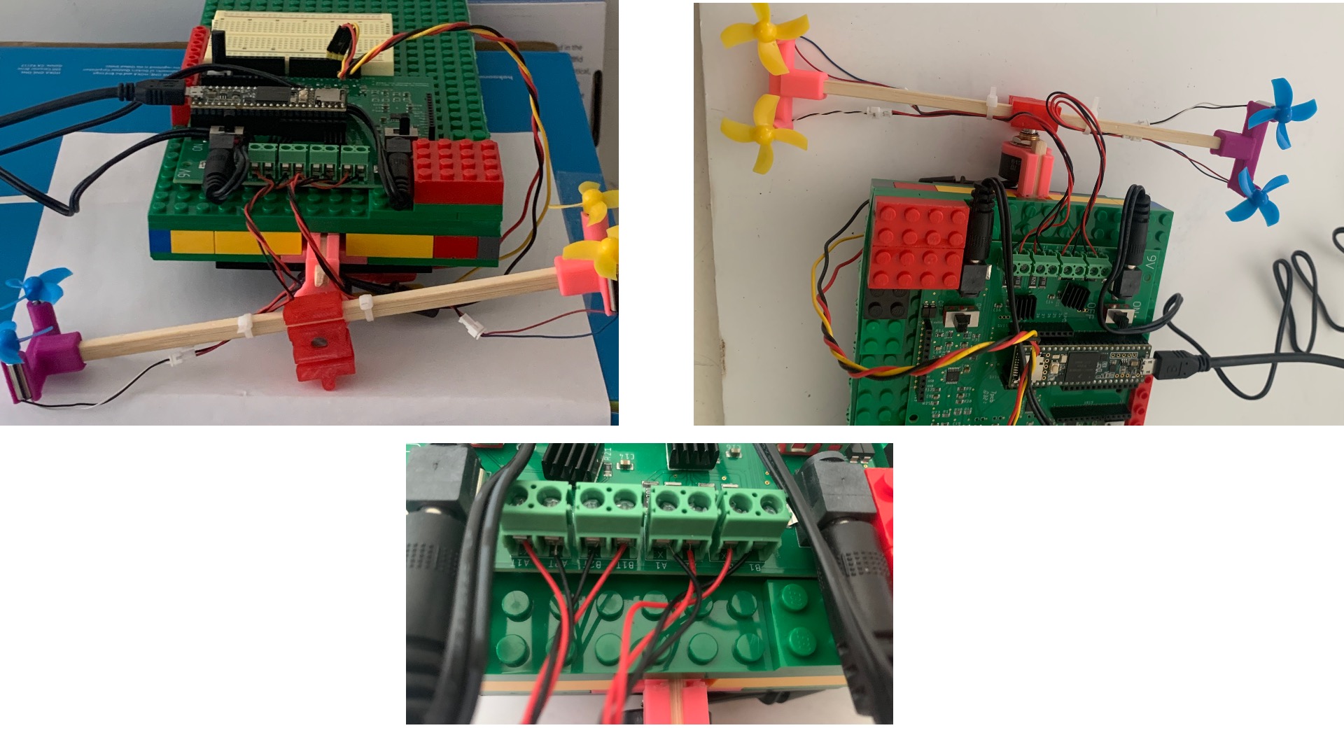
You've already constructed a two-propeller arm, for the resonance lab, but just like last week's state-space modeling, you should be as in the images in the picture below.

The details for how to wire the propeller for parallel drive, as shown in the figures below.

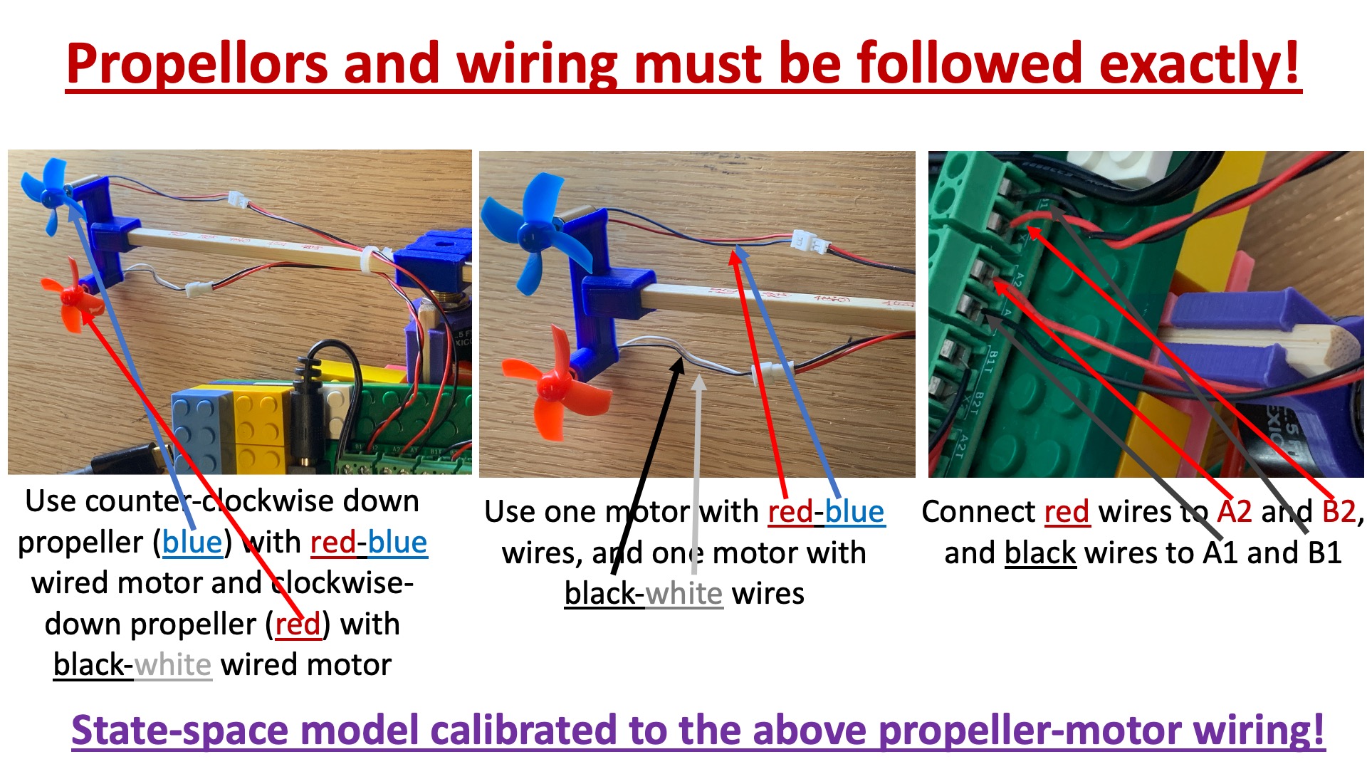
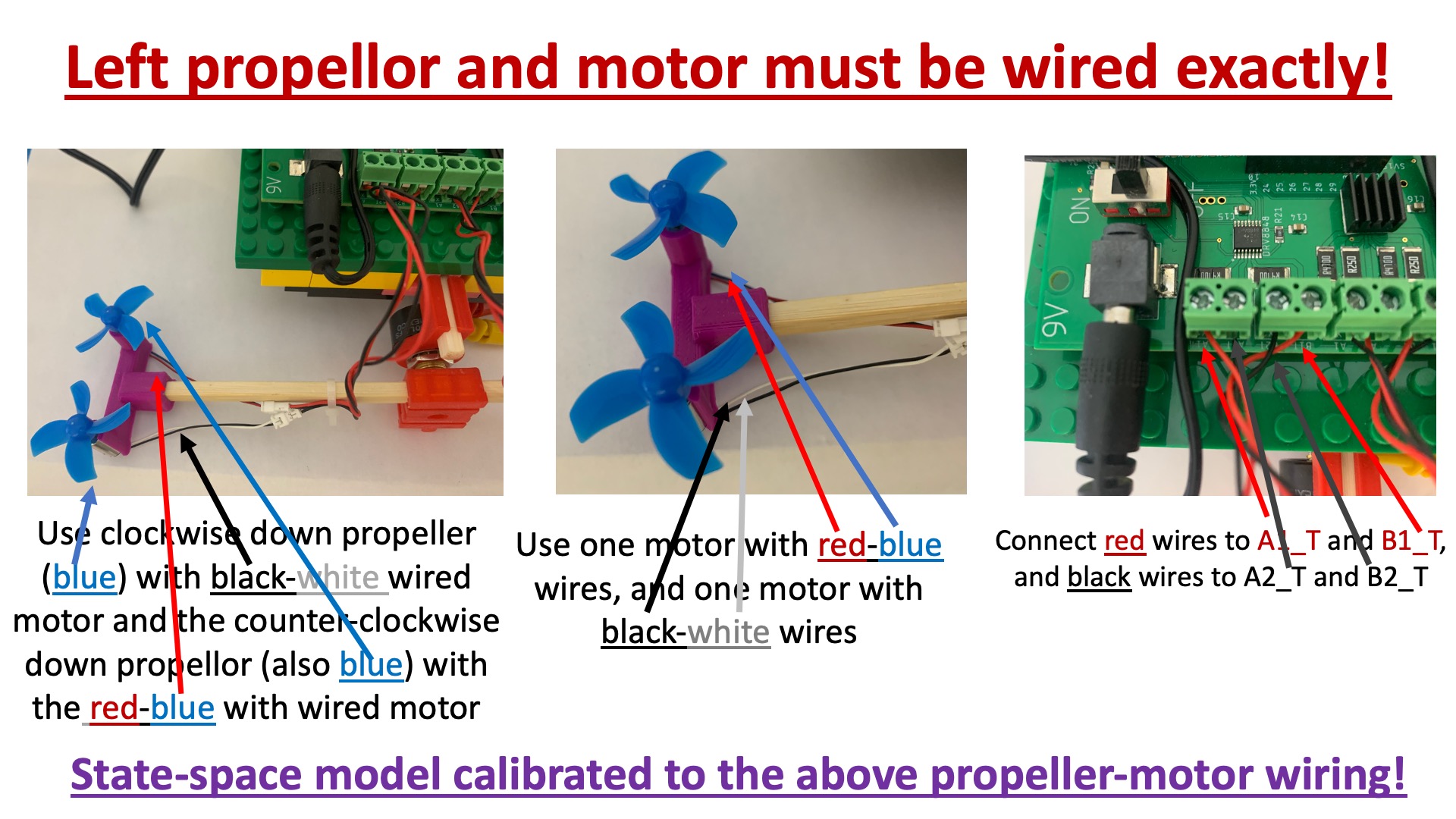
Make sure that the left propeller is wired to the left screw terminals and the right propeller is wired to the right screw terminals, as shown in the image below.

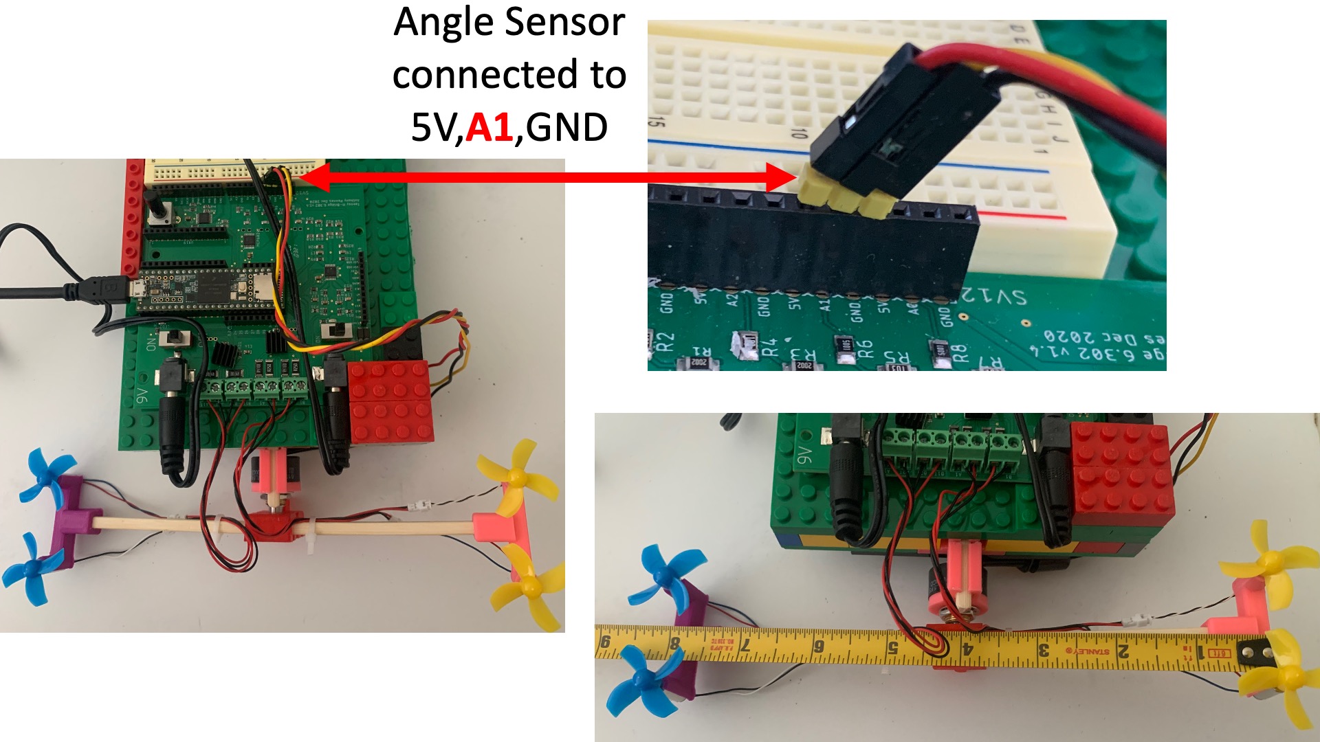
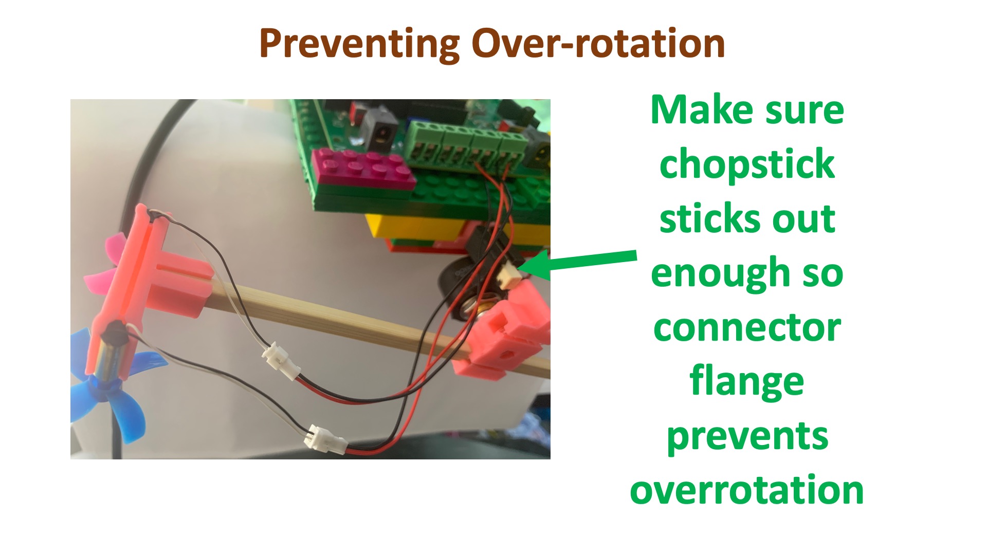
The two-propeller arm can rotate much faster than the single prop arm, and will rip out the wires if it starts spinning out of control. To prevent this, make sure that the chopstick connecting the angle sensor holder to the base plate protrudes enough to prevent the arm from rotating more than 180 degrees. See the figure below.

2.4) The software

The matlab scripts and the Teensy sketch to support this lab are all in one zip,

HERE.

IT IS ESSENTIAL that you keep all the files from the above zip in same directory, so that any updates you make to the matlab-based state-space model or to the controller can be transferred automatically to the Teensy. Automating the transfer makes it easier for you to "miss" some of the control design details, but eliminates the tedious and error-prone process of copying controllers by hand. Since this lab requires you to design many controllers, and we want you to explore alternatives, automation seemed to be the right tradeoff.

To use the automatic transfer, make sure that UseMatlabGenFile is set to true at the top of the Teensy 6302_Obs_Fall21 sketch. Then run the matlab script propSS.m to simulate your model and controller, and plot the results. The script also generates a human-readable file containing a definition of your controller, obs6302.h. When you compile and download the sketch 6302_Obs_Fall21 on to the Teensy, the compiler will read in the obs6302.h file, and download your controller on to the Teensy. DO NOT MANUALLY EDIT obs6302.h IN ARDUINO.

2.5) Using On-line Matlab.

Download and install MATLAB Drive Connector, which can be downloaded from the MATLAB Drive page. Matlab drive connector allows you to keep a local synced copy of the files you edit in on-line matlab.

To use matlab drive connector, download and install it, and then start matlab connector. Then download the zip file for this lab, and copy it into a directory on your local matlab drive. Unzip the file, and then you should be able to see a directory containing the Teensy sketch and the matlab files. Try clicking on the propSS.m matlab file and it should open in Matlab.

Use Teensyduino to open the 6302_Obs_Fall21 sketch in the same directory as the propSS.m you just openned. If the matlab connector is working properly, when you run propSS.m in the on-line matlab, the syncing should update your local version of obs6302.h. Then when you compile and download the 6302_Obs_Fall21 sketch from the local matlab drive on to the Teensy 3.6, it should pick up the synced, updated, obs6302.h file.

2.6) Initial Testing and calibration

Make sure the useMatlabGenFile is false in the Teensy 6302_Obs_Fall21 sketch, and then flash it on to the Teensy. Then start the serial plotter, and turn on the power to both propellers, and you should see multiple plots, like in the picture below. The plots show, from bottom to top, the desired angle, the measured and estimated three propeller-arm states (theta, omega and backEMF), and the motor command. The arm should be level, the plots should have the angle being zero, and the backEMF should be zero (matching the flat lines of the estimated states which are all zero).

Below is an uncalibrated system, showing the angle and BackEmf mismatches.

After you adjust the theta offset, the nomCmdL and nomCmdR, and the nomBemf, lines 17->20, you should see a calibrated plot, like the one below.

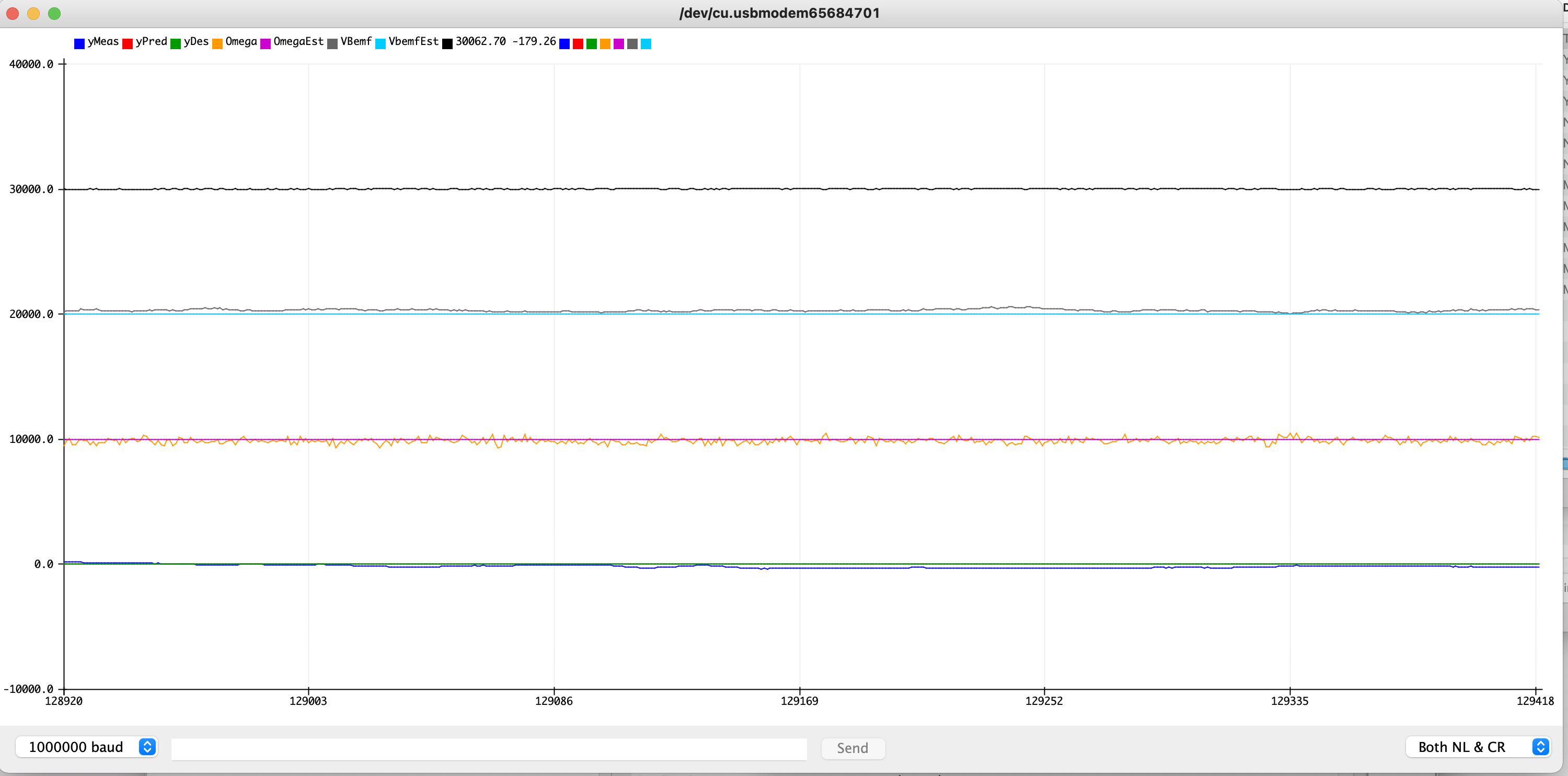
If you set the UseMatlabGenFile to true on line 14 in the Teensy sketch, run propSS.m unmodified, then flash the Teensy with the 6302_Obs_Fall21 sketch, and turned on the power to BOTH propellers (once you have verified they are both blowing down), then you will be able to run a default controller (once you have calibrated your system). If you type "1 0.1" in the entry window on the serial plotter, and you've calibrated the angle offset and nominal values, you should see the plot shown below.

2.7) Calibration

Note that you should recalibrate every time you start working with the arm, as the propeller does change over time, and calibrating with a low gain PD controller is quick and reliable.

2.7.1) Angle Offset and nominal values.

First lets recalibrate the angle sensor and set nomCmd1 and nomCmd2 to hold the arm horizontal. In the Teensy 6302_OBS_FALL21 sketch, when you set the UseMatlabGenFile flag at the top of the Teensy file to false, it will use its default parameters for a low-performance PD controller (on lines 40 and 41 in the Teensy code).

Place your two propeller setup so that the arm is free to rotate, make sure that the UseMatlabGenFile flag at the top of Teensy 6302_Obs_Fall21 sketch is set to false, flash the Teensy 3.6, start and start the serial plotter. Then use the following steps to set the angle offset and the nominal values for the commands and the backEMF.

• Step 1: With the propellers turned off, set thetaOffset so that the angle plot reads exactly zero when you hold the propeller arm (with your hand if necessary) exactly horizontal.
• Step 2: While holding the arm horizontal, turn on both propellers and verify each propeller is blowing air downwards (place your hand underneath).
• Step 3: Rotate the arm and verify that the propeller above horizontal slows down and the propeller below horizontal speeds up. If not, make sure the propeller on the left is connected to A1T->B2T terminals, and the propeller on the right is connected to A1->B2 terminals. Ask for help if you are unsure!
• Step 4: Let go of the arm, and it should hold itself near horizontal.
• Step 5: Slightly symmetrically increase or decrease cmdNomL and cmdNomR in the Teensy sketch if the arm is not holding itself exactly horizontal. A reasonable cmdNomL is between 0.45 and 0.55, and cmdNomR, 0.55 and 0.45 (move the left up the same amount you move the right down). if you need a higher or lower value, then something may be wrong with your propeller. Ask for help!
• Step 6: If you correctly determined thetaOffset, cmdNomR, and cmdNomL, the arm should be holding itself perfectly horizontal, and yMeas should read zero (and match yDes). *Step 7: Adjust the nomBemf value so that the vBemf plot (second from the top) is zero (matches the estBemf line).

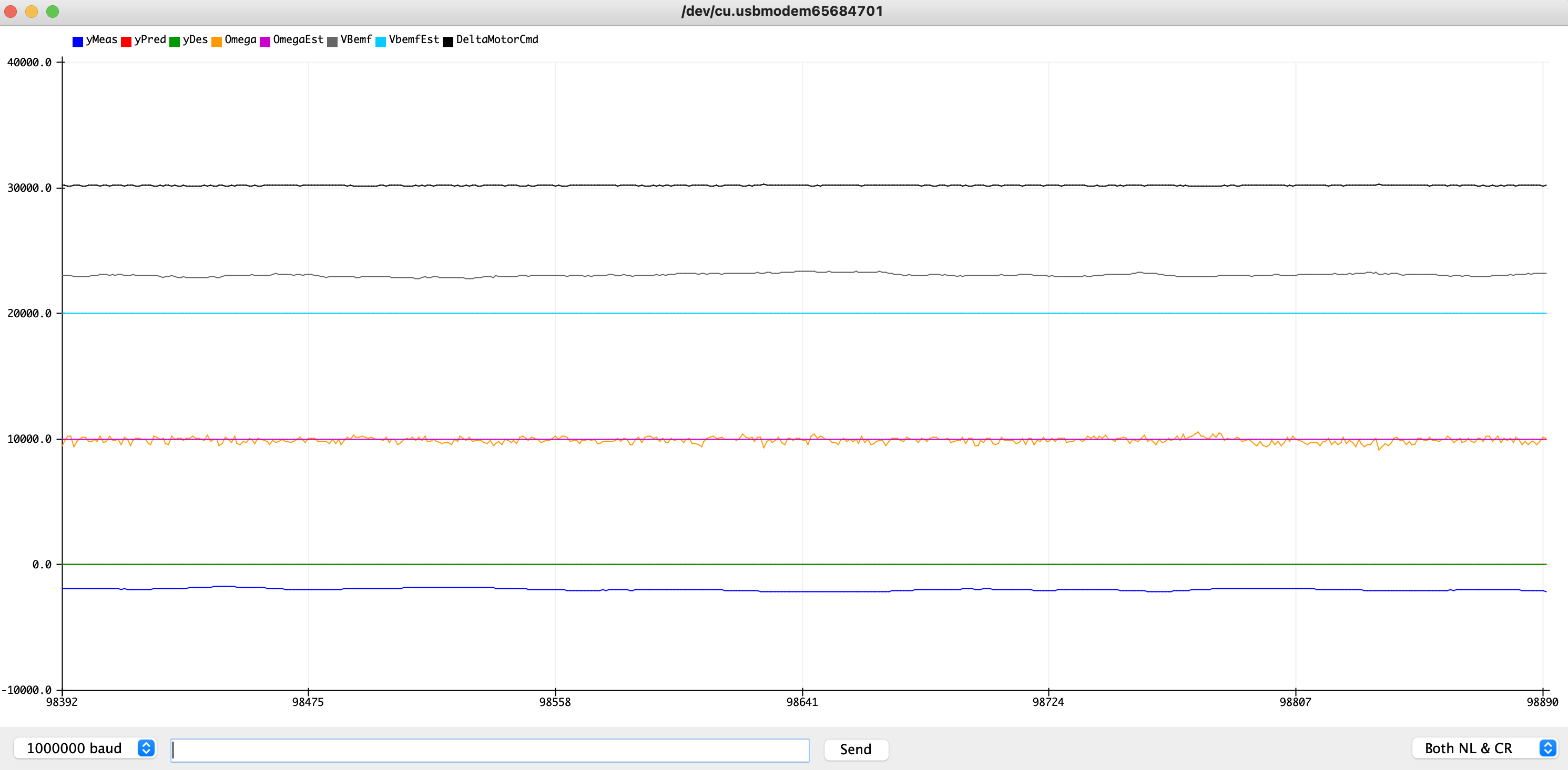
Once you have calibrated the nominal values and the angle sensor, your plots should look like the image below Note that all the plots should be zero, but there is measurement noise on both the Omega and backEMF plots.

2.7.2) Calibrating the state-space model.

Test the automatic transfer from matlab to Teensy by setting the UseMatlabGenFile flag at the top of the 6302_Obs_Fall21 sketch to true, and changing the PD controller gains in matlab by updating the Kd vector (near line 25 of the dtObs.m matlab file) and Krd (near line 30). Run propSS.m in matlab, then flash the Teensy 3.6 with 6302_Obs_Fall21, and see if the gains you set in the dtObs.m file cause a change in the behavior of the arm.

Once you have verified that changes in matlab are making their way to the Teensy, you can compare simulated and measured step responses for your propeller under low-gain PD control. Try a proportional gain of 2, and a derivative gain of 0.5, and then try reducing the derivative gain to 0.25 (in each case by changing the Kd vector in matlab, and then updating the controller on the Teensy by rerunning propSS.m, and reflashing with the 6302_Obs_Fall21 sketch).

You will likely see that the measured behavior of the propeller arm is either more stable or less stable than predicted by the simulation. One way to improve the match by adding arm friction to the matlab state-space model in propModel.m (note that the model already has MOTOR friction, but not ARM friction). Where will you put the arm friction? What if your model is more stable than the arm? Then you can try to improve the match by adjusting, depending on the mismatch, the motor rotational inertia, using tweakJm, and the arm rotational inertia, tweakPropM, both at the top of the model file, propModel.m.

Be sure to test your modifications to propModel.m for several different angle-step sizes (by setting the stepsize to different values), but carefully monitor the motor command plot (top plot). If the motor command "saturates", then your linear model will not match, regardless of your modifications.

3) Checkoff 1

In this first checkoff you will wire up a two-propeller arm, calibrate its controller, tweak an associated state-space model to improve matching, and then use LQR to determine DT state-space controller gains.

In particular, please:

• Attach the second propeller to make a two-prop arm as shown above.
• Download the software for this week, run the matlab file propSS.m in the 6302_OBS_FALL21 directory, upload the 6302_OBS_Fall21 sketch to the Teensy 3.6, and start the serial plotter.
• Calibrate your arm's angle sensor offset, nominal command, and nominal backEMF, as described above.
• Improve the match between your arm and the matlab model in propModel.m, as described above. Add arm friction to the state-space model and adjust other model parameters as needed to improve the match between the matlab simulation and your arm.
• You should find all the lines in dt2obs.m that say FIX THIS that occur before the observer section (Ldplace is defined at the beginning of the observer section, you will fix that section in checkoff 2), and fix them, EXCEPT lines 20->22, those lines refer to using LQR when the model is generated numerically using a fitter, and that is in checkoff 3. In particular, you should be careful about Krd, whose derivation you can find in the 5/11 lecture scribbles.
• Determine feedback gains by setting good LQR weights. In discrete-time, the matlab function is dlqr, but the weights have the same meaning as in continuous time, so you can start with the weights you determined for the single prop arm.
• Run the propSS.m script to simulate your model and controller, and see if your weight adjustments had the intended effect. You should only look at the plots of the measured-state feedback, you will look at the estimate-state feedback plots in checkoff 2. Remember that the script also generates a human-readable file containing a definiton of your controller, obs6302.h.
• When testing a controller on the propeller arm, flash the sketch 6302_Obs_Fall21 on to the Teensy. Be sure you run propSS.m in matlab first, which generates the obs6302.h file that the Teensy compiler will read, and download your latest controller on to the Teensy.
• Try adjusting the scale factor on NoiseAmps (on line 42 in propSS.m), and rerun the script (this does NOT change the obs6302.h file, it only changes the simulation). What happens to the matlab plots for the measured-state feedback system (you have not set up the estimated-state feedback system yet, so ignore those). Why is NoiseAmps, on line 42 in propSS.m, a scaled length-three vector?

Checkoff 1:

YOU MUST BE ABLE TO ANSWER ALL THE CHECKOFF QUESTIONS IN ORDER TO GET THE CHECKOFF!!!

1. Show that your arm is calibrated
2. Show that the gains are being updated in the teensy code after you run the matlab script
3. Describe how you added friction to the state-space model. How did you determine if it was necessary? What other parameters did you change?
4. Demonstrate a good match between simulation and experiment
5. Explain all the fixes made to dtObs.m
6. Finally, you should be able to explain what happens when you turn on the noise modeling. How well does the noise in the simulation match the noise you see?

Ask for Help Ask for Checkoff

4) Checkoff 2

For this checkoff, you will determine gains for observer-based state estimation, and use them for your controller. The key issues will be ensuring fast convergence of the state estimates, while keeping the noise low. You will be able to simulate the behavior in matlab before trying it on the arm, but the simulation does not include all the non-idealities of your propeller-arm system, and does not include the realistic disturbances (like wind gusts, or the propeller hitting the edge of the table, etc), so its simulation of state estimate accuracy will be informative, but probably optimistic.

4.1) Determining observer gains.

As part of this checkoff, you should find all the lines in dt2obs.m associated with the observer that say FIX THIS and fix them. But to fix the observer part of the dtObs function, you will have to decide how to pick observer gains, the Ld's. You want to ensure fast convergence of the state estimates, as those estimates will be used in the state-feedback controller.

You must decide how to use matlab's place function to compute the Ld's, but its application is not that straight-forward. You should think carefully about the fact that the estimator gains depend on Cd, but Cd is the wrong shape for dlqr and place (Cd is 1x3, but Bd is 3x1). And both dlqr and place return K's, which are also the wrong shape (Kd is 1x3, Ld is 3x1). The matlab tick (') command transposes matrices, so Cd' is the transpose of Cd, but Cd is not the only matrix you will need to transpose. And you might find the following transpose identity useful,

Once you have a strategy for determining estimator gains, run the propSS.m script to simulate your model and controller, and see if your changes had the intended effect. Try setting the perturb flag to true at line 16 at the top of the propSS.m file, and rerun the simulation. Do you see a change? The perturb flag causes the simulator to zero out the estimated state about 3/4's of the way through the simulation, to make it easier to see how fast the estimation converges. Then try adjusting the noise model (on line 42 in propSS.m), and rerun propSS.m. How does the resulting noise depend on the estimator gains? What if you try to force the estimates to converge very fast, what happens to the noise?

4.2) Running the controller

When you are satisfied that you have good gains, be sure that flag UseMatlabGenFile is set to true (the biggerStep flag should still be false) at the top of the 6302_Obs_Fall21 sketch. Then run the propSS.m script, as it will generate a human-readable file containing a definiton of your controller, including the estimator gains and new state-space model. Then compile and download the 6302_SS_control sketch on to the Teensy.

Once your controller is downloaded, try setting the step size to 0.05 (a small step), and compare the estimated states to the measured states in the top three plots (the red and blue curves). Do they match well? What happens when you set the 0.2 step (a bigger step)? If the motor command saturates (see the top plot in the plotter), are your state estimates accurate? Look at lines 300-311 in the Teensy sketch, where the state estimates are computed. Can you move a few lines of code so that the estimator is more accurate when the motor command saturates?

To quickly compare estimated-state feedback to measured-state feedback, type "3 1" or "3 0" in the plotter entry window. What changes when you switch back and forth? Which is better and why?

4.3) Checkoff 2 step-by-step

• Be sure that flag UseMatlabGenFile is set to true (and the biggerStep flag should still be false) at the top of the 6302_Obs_Fall21 sketch.
• You should find all the FIX THIS lines in dt2obs.m associated with the observer, starting with the line that defines LdPlace and ending with the beginning of the integral term (adding the integral is interesting, but definitely optional), and fix them.
• You will have to decide how to pick the gains for converging the observer estimates, the Ld's, using matlab's place command, but you should think carefully about what those commands take as input, and what they produce as output. The estimator gains should depend on Cd, not Bd, but Cd is the wrong shape (Cd is 1xn, but Bd is nx1). Also, place and dlqr return feedback feedback gains, which are the wrong shape (Kd is 1xn, Ld is nx1). The matlab tick (') command transposes matrices, so Cd' is the transpose of Cd, but Cd is not the only matrix or output you will need to transpose.
• Run the propSS.m script to simulate your model and controller, and see if your changes had the intended effect. Try setting the perturb flag to true at the top of the propSS.m file, and rerun the simulation. Do you see the change? The perturb flag causes the simulator to zero out the estimated state about 3/4's of the way through the simulation, to make it easier to see how fast the estimation error decays.
• Try setting NoiseScale to 1.0 (on line 17 in propSS.m), and rerunning propSS.m. How does the resulting noise depend on the estimator gains? What if you try to force the state estimates to converge very fast, what happens to the noise?
• Once again, the script generates the file obs6302.h which contains the definiton of your controller, including the observer model and the estimator gains. So when you compile and flash the sketch 6302_Obs_Fall21 on to the Teensy, the compiler will read in the latest obs6302.h include file, and download your controller on to the Teensy, including the observer model and the estimator gains.
• Pick "good" Kd's and Ld's, run propSS.m, then download 6302_Obs_Fall21 on to the Teensy, start the serial plotter, type "3 1" and then "1 -0.05" in the plotter entry window, to use estimated states and a small step size. Compare the estimated states to the measured states in the plots. Do they match well? Try other step sizes.
• What happens when you set the step size to 0.5 (a big step, type "1 0.5" in the plotter entry window)? If the motor command saturates, are your state estimates accurate? Look at lines 301 through 310 in the Teensy sketch, where the state estimates are computed. Can you move a few lines of the code so that the estimator is more accurate when the motor command saturates? Look for where the u's are beginning clipped (near line 315 in the Teensy sketch).
• You can quickly compare estimated-state feedback to measured-state feedback by typing "3 1" or "3 0" to using estimated or measured state, respectively. What changes when you switch back and forth? Which is better and why?
• Got a good controller? Are you Brave? Try using step-sizes close to 2.5!

Below is a video of one of our estimated-state feedback controllers from last Spring.

Checkoff 2:

YOU MUST BE ABLE TO ANSWER ALL THE CHECKOFF QUESTIONS IN ORDER TO GET THE CHECKOFF!!!

1. Explain all the fixes you made to dtObs.m
2. Explain how you picked estimators gains
3. Explain how noise performance relates to estimator gains
4. Explain what you changed in the Teensy sketch and why
5. Demonstrate different controllers on your propeller arm. Can you achieve performance like our video?
6. When you switch between estimated-state and measured-states feedback, is the performance better or worse, and what about the noise?

Ask for Help Ask for Checkoff