Tools for Manipulating Transfer Functions.

The questions below are due on Tuesday October 05, 2021; 09:00:00 AM.

You are not logged in.
Please Log In for full access to the web site.
Note that this link will take you to an external site (https://shimmer.mit.edu) to authenticate, and then you will be redirected back to this page.

This question is meant to show you how to use transfer function representations, plus a good software package, to build up complex system descriptions by composing. The examples below use MATLAB, but many of the functions are also available in the python controls package. Come to office hours or post on Piazza if you have problems and we'll help.

Most of the packages for manipulating transfer functions are much better at manipulating transfer functions that are specified as ratios of polynominals in z rather than z^{-1}. For example, using the shift-and-scaling identity for the Z transform, we would transform the difference equation

x[n] = a x[n-1] + b w[n-1]

X(z) = a z^{-1} X(z) + b z^{-1} W(z)

X(z) = H(z) W(z) \;\; = \;\;\frac{bz^{-1}}{1 - a z^{-1}} \;\; W(z) .

As long as z is not zero, we can rewrite H(z) as

H(z) = \frac{bz^{-1}}{1 - a z^{-1}} = \frac{b}{z - a},

where the rightmost form is the one MATLAB manipulates most readily.

In MATLAB, you can manipulate discrete-time transfer functions using z if, at the beginning of your session you type:

>> z = tf([1 0], [1], -1)

The above command informs matlab that z is a discrete-time transfer function. BE SURE TO INCLUDE THE -1 IN THE tf() COMMAND, IT INFORMS MATLAB THAT THIS IS A Discrete-Time TRANSFER FUNCTION with a GENERIC sample period. You can also replace the -1 with 0.001 if you only plan to consider one millisecond sample periods. And if you do, then the x-axis for your plots will be time in seconds, rather than sample indices. For example, if \Delta T = 0.001, use

>> z = tf([1 0], [1], 0.001)

Once you have specified that z is a transfer function, arithmetic operations involving z will also produce transfer functions. For example, if you type:

>> Gamma = 10; dt = 0.001; Hsys1 = Gamma * dt * dt * (1/(z-1))*(1/(z-1))

Matlab will respond with the following:

Hsys1 =

      1e-05

  -------------

  z^2 - 2 z + 1


Sample time: unspecified

Discrete-time transfer function.

We are often interested in how increasing overall controller gain affect the transfer function of the closed-loop feedback system:

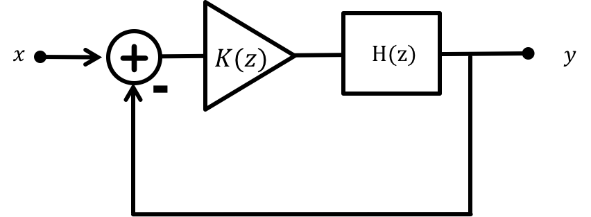
where in this case, H(z) = H_{sys1}(z) above, K(z) = K_0 K_n(z) where K_0 is a scalar representing overall controller gain and K_n(z) is a normalized controller. Black's formula yields the closed-loop transfer function, G, where

G = \frac{K_0 K_n(z)Hsys1(z)}{1 + K_0 K_n(z)Hsys1(z)},

though there is a subtlety about how to compute G as we will see below.

To plot the poles (or natural frequencies) of G as a function the scalar gain K_0, assuming K_n(z) = 1 in the above formula, in MATLAB type

>> rlocus(Hsys1)

and you will see the root locus below.

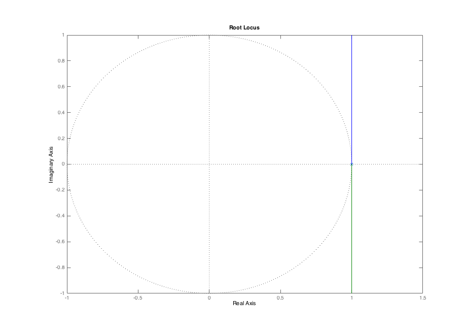
If you defined z using tf as above, then you can use z to define a PD controller transfer function. For example, consider proportional and delta (aka derivative) gains, denoted Kp and Kd respectively, for a PD controller representerd by the difference equation relating error, e[n] to actuator command, c[n],

c[n] = K_p e[n] + \frac{K_d}{\Delta T} (e[n] - e[n-1]).

Using Z transforms, we can express the PD transfer function as

C(z) = K(z) E(z) = (K_p + \frac{K_d}{\Delta T}(1 - z^{-1})) E(z),

K(z) = (K_p + \frac{K_d}{\Delta T}\frac{z - 1}{z}).

where note that we have replaced 1 - z^{-1} with \frac{z-1}{z} because Matlab is not as facile at manipulating z^{-1}

To generate a MATLAB transfer function for a PD controller with specific values of K_p and K_d, type, for example

>>  Kp = 1.0; Kd = 0.5; Kpd = Kp + Kd/dt * (z-1)/z;

To determine the closed-loop transfer function G for the feedback system with controller K_{pd} and plant H_{sys1} , we can execute the matlab command

>> G = feedback(Kpd*Hsys1,1)

and see a plot of the closed-loop step response with the command

>> step(G);

If you specified a sample interval when defining z using the tf command, For discrete-time systems specified using a GENERIC sample rate, -1, in the example near the top of the page, matlab's step function assumes a sample period of one second. Our sample period is one millisecond, so you can interpret the time axis as being in milliseconds.

Instead, if you specified the real sample interval in the tf command, then you can set plot intervals using real time. For example,

>> step(G,5);

will plot 5 samples if you used -1 to define z using the tf command, and will plot 5000 samples, or five seconds, if you used 0.001 in the tf command.

Note that feedback(Kpd * Hsys1,1),with 1 as the second argument, returns the closed-loop transfer function for what we often refer to as a tracking feedback system. That is, the matlab function feedback returns a transfer function that is equivalent to

G = \frac{K(z)H(z)}{1 + K(z)H(z)}.

Since Black's formula is simple enough, why don't we just use that? Why do we need a special feedback function? For our PD controller example, we could compute G using the matlab command

>> G = (Kpd*Hsys1)/(1+Kpd*Hsys1)

but the returned transfer function would not be identical to the result from the feedback function. Try both approaches to computing G using Matlab, and then determine the differences between the two closed-loop transfer functions. What is the difference between the two?

What is the difference between G computed using Black's formula explicitly, and G computed using the feedback function?

There are extra poles, the poles of Hsys

There are extra zeros, the zeros of Hsys

There are extra poles equal to the poles of Hsys, and extra zeros equal to the poles of Hsys

There are extra poles and zeros that exactly cancel

If we are given dt = 0.001 and Gamma = 10, suppose we set Kp = 1 (to normalize for the root locus plot), and guess at a good value for Kd (maybe start with 0.2, but for this problem you don't know what "we" selected), and then type

>> Kd = 0.2, Kp = 1.0, dt = 0.001; Gamma = 10; Hsys1 = Gamma*dt*dt*(1/(z-1))*(1/(z-1)); Kpd = Kp + Kd/dt*(z-1)/(z); rlocus(Kpd*Hsys1);

Can we determine the value of K_d from looking a the resulting root locus plot? Not really, because the important details are crowded around the point z = 1. If you do not see the plot, try typing Matlab's show graph command:

>> shg

root locus

We can focus on the details around z=1 by using the command

>> rlocus(Kpd*Hsys1, linspace(0,10,1000))

which plots the poles for the closed-loop system

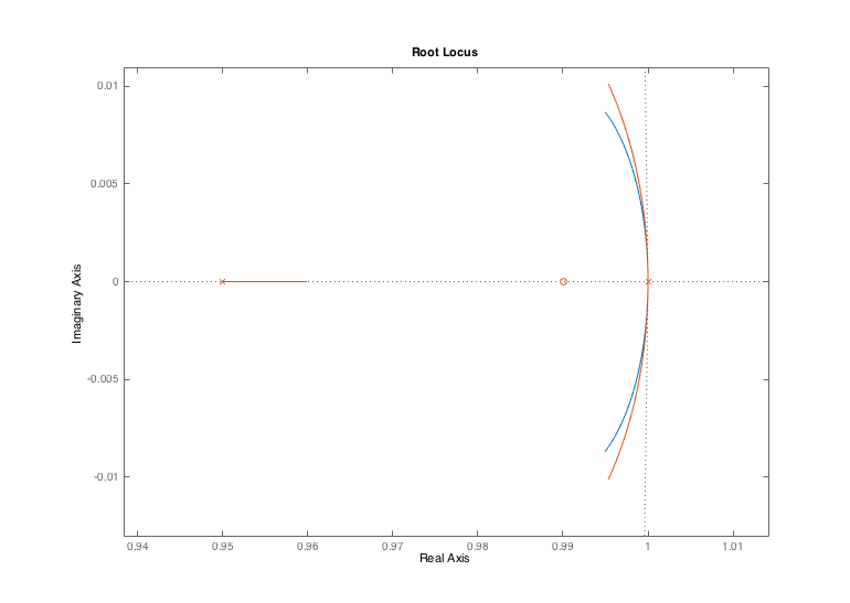
\frac{K_0\cdot K_{pd}\cdot H_{sys1}}{1 + K_0\cdot K_{pd}\cdot H_{sys1}}

for one thousand values of K_0 between 0 and 10.

By looking at the root locus, and zooming in as in the figure below, you can see enough important details to estimate the value of K_d, to at least one digit (try redrawing the zoomed-in root locus plot for K_d = 0.3, 0.4, ...).

root locus

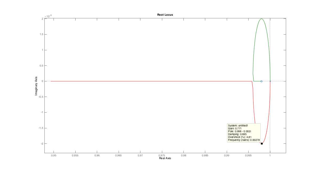
What value of K_d yields a root-locus plot matching the one shown in the screenshot above.

What is the value of K_d?

An Extra Pole

Suppose we consider adding an additional pole to our model for the system, that is,

>> Hsys1p = ((1-0.95)/(z-0.95))*Hsys1;

We can then compare the impact of the new system model using matlab's rlocus command, as the command takes multiple transfer functions. That is, we can compare the root locuses for the two cases with

>> rlocus(Kpd*Hsys1, Kpd*Hsys1p, linspace(0,10,1000))

The zoomed in root locus for the plot is shown below (from matlab), please use it to answer the questions below the figure. You will have to use trial and error with K_d again.

root locus

Is the blue root locus for Hsys1 or Hsys1p?

Hsys1p

Hsys1

What is the value of K_d?

Using K_p = 1 and K_d equal to the value you just found when comparing the two loci, let's consider what happens when we scale both K_p and K_d by K_0 . In particular, what is the maximum value for this scale factor, K_0, so that the closed-loop system involving Hsys1 has the same frequency of ringing in its step-response as the closed-loop system involving Hsys1p (to within five percent).

Trial and error, with an educated guess at the good trial values, is about the only way to find K_0, so do not worry about getting K_0 to better than to better than 5 percent. You may find it helpful to use the matlab command

>> pole(G)

and look at the imaginary parts (be sure to type "pole", do NOT make it plural).

Maximum value of K_0 so that the two systems have the same oscillation frequency in their step response?

Suppose the location of the extra pole 0.98, closer to one, which we can generate with the matlab command

>> Hsys1p = ((1-0.98)/(z-0.98))*Hsys1;

For this slower system, we expect worse ringing, and therefore we expect a lower maximum for K_0, but by how much?

does your answer to the prevous question change to a K_0 less than three?

yes

does your answer to the prevous question change to a K_0 less than one?

yes

One might wonder why root locus plots are given so much importance. They trace the natural frequencies of the feedback system as a function of a single scale factor K_0, but a PD controller has two gains, a PID controller three. Why is one particular plot of natural frequencies versus scale factor so important, and why should it be the one that maintains gain ratios? For example, why not plot the natural frequencies of a feedback system as a function of K_0 given a controller with a fixed proportional gain,

K(z) = (K_p + K_0\frac{K_d}{\Delta T}\frac{z - 1}{z}),

or with a fixed derivative gain,

K(z) = (K_0 K_p + \frac{K_d}{\Delta T}\frac{z - 1}{z}).

The answer is largely historical. Adjustable gain amplifiers have always been simple to build, so putting one in series with a controller was a easy parameterization. Note that the matlab script at the beginning of the PD control exercises can be used to create a variety of locus plots, a swarm of locuses, one might say.