Fan Example
Please Log In for full access to the web site.
Note that this link will take you to an external site (https://shimmer.mit.edu) to authenticate, and then you will be redirected back to this page.
Suppose we are designing a fan-speed algorithm for a micro-controller and we have two inputs, the desired fan speed, w[n], and the sensed fan speed, v[n], and one output, c[n], the fan motor current. As usual, n is the sample index. Our design problem is to determine how to set the motor current given the desired and sensed fan speed.
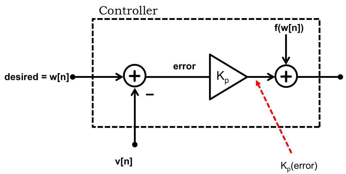
 Diagram of the Fan Speed Control with Proportional Feedback.
As a first attempt, our controller design uses proportional feedback, as shown in the figure above. We compute the speed error, e[n] as the difference between the desired fan speed and the measured fan speed,
The problem: The fan has a lot of friction and air resistance, so a high motor current is needed to keep the motor spinning at the desired speed. But the only way our proportional feedback controller will set the motor current to a high value is either: (1) K_p is large, or (2) the error in fan speed is large. Our micro-controller does not sample that fast, and we now know that the system will become unstable if the gain is too high. With a slow sample rate, the limit on the gain is low. So we are stuck, we have to accept a large fan speed error.
We would like to reduce the constant error term. To do so, we will accumulate the error over time and add this term to the motor current. That is,
where the sum term is normalized by the sampling interval. The proportionalty constant for this term is called K_i as this sum is a discrete time approximation of a continuous time integral.
The reason for the sum term is that if the fan speed is consistently too slow, then the sum of the fan speed errors will accumulate, and K_i \Delta T \sum _{m=0}^{m=n} e[m] will continue to rise until the motor current is high enough to make the fan spin at the desired speed.
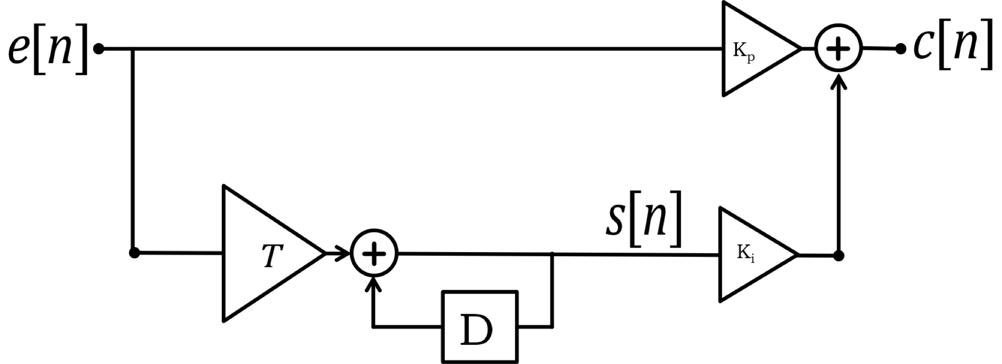
The sum term looks like it will do the job, by continuing to increase, and therefore causing the fan motor current to increase, until the needed corrections are made to the fan speed. But, it looks like the sum term will be expensive to compute, because we will have to sum all of the past errors every timestep. How can we compute this sum, which we will denote as s[n], without storing the entire past history of errors? And how can we avoid adding up all those past errors each time?
There is an efficient and elegant approach to the summation problem, using an LDE of course! That is,

In the figure above, we show a block diagram representation of the proportional plus sum fan speed controller. In the figure, you will notice a block marked D , which we use to note a one-sample delay. Finding block diagram approaches to representing LDEs can help organize the important effects in a complicated system. For example, we can see that error at the present step is scaled before being added to the sum, and that it effects the sum immediately (there is no delay block in its way).
Problem: The motor current is responsible for both overcoming friction and accelerating the fan. So if the fan starts at zero speed, then for the fan speed to reach the desired speed, the motor current must exceed the current needed to maintain the desired speed. If K_p is small, then that very high motor current is primarily due to the sum term alone, c[n] \approx K_i s[n]. Since the sum term decreases only if the speed errors are negative, or when the fan speed is higher than the desired speed, it will keep the motor current high enough to accelerate way past the desired speed.
Once the fan speed exceeds the desired speed, the errors change sign, and the K_i s[n] term starts to decrease. And if all goes well, the sum term should settle on a value that produces just enough motor current to overcome friction and air resistance. But, either K_i is set to a very small value, in which case achieving the desired speed will take a long time, or K_i is set to a large value, and the fan speed substantially overshoots the desired speed. That is, the fan speed accelerates until it is spinning too fast, and then decelerates to the desired speed. And if K_i is very large, the system will become unstable, in which case the fan speed would probably oscillate back and forth from zero to its maximum speed, until the motor breaks.
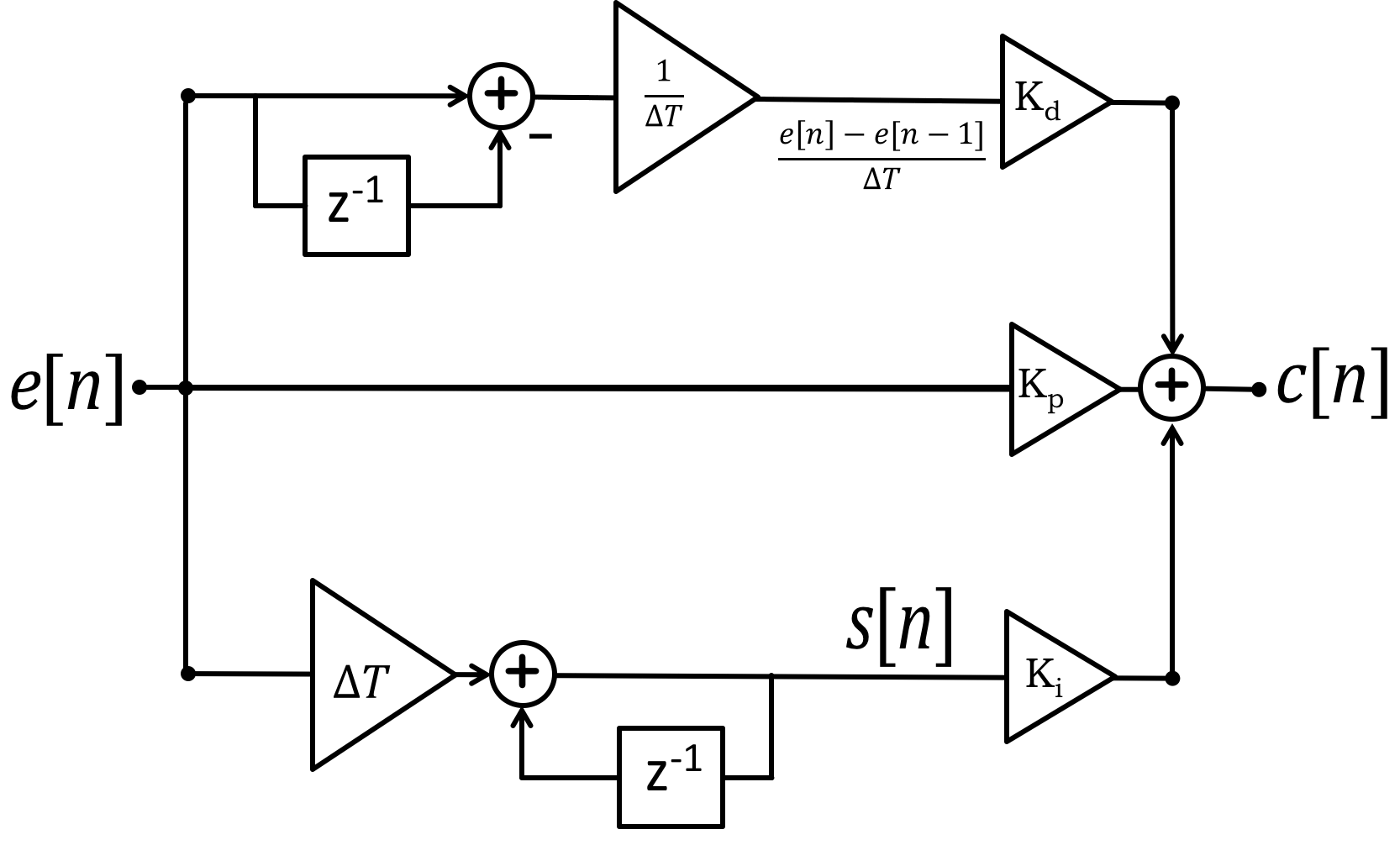
where we have introduced a normalization for the Delta term by dividing the change in error by the time between error samples, T, motivated by analogy to its continuous-time equivalent, the derivative.
This new Delta term is negative if the new error is smaller than the old error, so it acts to decrease the motor current if the speed errors are decreasing too rapidly. The Delta term is roughly equivalent, in this case, to the negative of the fan acceleration. It acts to balance the increasing acceleration that would be produced by the integral term alone.

The controller we have just developed is usually called a Proportional-Integral-Derivative (PID) controller, but since it is almost always implemented with a micro-controller in discrete time, a more accurate label would be a Proportional plus Sum plus Delta (PSD) controller.
In the PSD controller shown above, the new part of the block diagram is at the top, and is used for computing the delta term in the controller. Note that for the top part, the input to the delay block is before the subtractor, so the delayed data is used once and then forgotten. Just as one would expect given the goal was to compute error differences. Compare the top part to the bottom part of the PSD controller, in which the sum term is computed. In the bottom section, the input to the delay is after the subtractor, so the results of the subtraction persists. Again, just as one would expect given that sums are cumulative.
From the above block diagram, the Z transform of e[n], \mathcal{E}(z), is related to the Z transform of c[n], \mathcal{C}(z), by the transfer function \mathcal{K}(z). That is,
Once you know A, B and C, can you write down the difference equation relating c[n] to e[n]?
In general, we can use a PSD controller and try to adjust the three parameters, K_p, K_i and K_d using our intuition about what the three terms do. We might even succeed in adjusting them so that the fan promptly accelerates to the desired speed, and does not overshoot. But to get the best values, and to make sure the controller is stable, we would have to form the difference equation for the entire controller. Then we could compute the natural frequencies of the difference equation as a function of the three PSD gains. And finally, we could adjust the parameters to minimize the maximum magnitude natural frequencies.
In this fan speed case, we are using feedback to create the high currents needed to overcome air resistance and friction, but these terms are primarily a function of desired speed, something we already know and do not need to measure.
So suppose we run a calibration sequence. That is, suppose we set the fan motor current to a sequence of 100 progressively larger currents, starting from zero and ending with the fan motor's maximum current. And after each change in fan current, we wait just long enough for the fan speed to settle to a steady value, and measure that speed. In this way, we can generate a table that relates motor current to fan speed, and we can also invert the table. That is, we can create a function, f, whose input is the desired fan speed, and whose output is the associated fan motor current.
To this function, f, created from inverting the current versus fan speed table, we can add just the proportional feedback term to trim off the errors in the table (and help accelerate the approach to the desired speed). That is, the motor current is
If we do a good job with our feed-forward approach, why do we still need feedback? Perhaps we need feedback because as the motor ages, its current versus speed function will change, and the feedback will correct those errors. But we could address that issue by, for example, recalibrating every time the fan is turned on?
But what if the fan is picked up and placed somewhere else in a room, perhaps right next to a wall, and the air resistance increases significantly. That is when we really need feedback, to keep the fan speed steady and reject the impact of disturbances.
