State of Op-Amps

The questions below are due on Friday November 26, 2021; 10:00:00 AM.

You are not logged in.
Please Log In for full access to the web site.
Note that this link will take you to an external site (https://shimmer.mit.edu) to authenticate, and then you will be redirected back to this page.

Connecting Transfer Functions to State Space: An op-amp example.

The operational amplifier, or the op-amp for the cognosenti, was an early, and remarkably successful, application of continuous-time control theory, and an essential component in most control systems. The first op-amp was introduced more than 80 years ago (using vacuum tubes), the modern op-amp (the 741, an integrated circuit) was introduced more than 50 years ago, and 20 years ago, at the end of the 20th century, the electronics industry consumed five billion op-amps a year. So, the op-amp has a well-deserved place in control theory's history, and is discussed in nearly every introductory class on control.

If op-amps are so important, why haven't we mentioned them earlier? The main reason is that fast microcontrollers, which can run sophisticated DT control algorithms, have displaced the use of op-amp-based CT controllers in all but the very highest frequency applications. For example, we used to have students implement a lead controller using an op-amp, three resistors, and a capacitor, but it is much easier for students to implement using a DT approximation on the Teensy.

Op-amps continue to play an extremely important role in signal processing, because an op-amp, plus a few resistors and capacitors, can implement a wide range of filters and amplifiers. But all those circuits rely on feedback principles, so one should learn a little about op-amps.

A little about op-amps

To understand op-amp theory, recall that when we started discussing continuous time, our first feedback example was the speed control problem. And we saw that when using proportional feedback, we could use any positive proportional gain, and the system would be stable. More precisely, suppose

\frac{d}{d t} ω_{m} (t) = - \Beta ω_{m} (t) + γ u (t),

where $ω_{m} (t)$ is motor speed, $\Beta$ is a friction coefficient, $u (t)$ is a control input, and $γ$ is a scaling coefficient. Then if $u (t)$ proportional to the difference between the desired ( $ω_{d} (t)$ ) and measured motor speed,

u (t) = K_{p} (ω_{d} (t) - ω_{m} (t)),

where $K_{p}$ is the proportional gain, then

\frac{d}{d t} ω_{m} (t) = - (γ K_{p} + \Beta) ω_{m} (t) + γ K_{p} ω_{d} (t),

and the response to an input step ( $ω_{m} (0) = 0$ and $ω_{d} (t) = 1$ for all $t > 0$ ) is a rising exponential

ω_{m} (t) = \frac{γ K_{p}}{γ K_{p} + \Beta} (1 - e^{- (γ K_{p} + \Beta) t})

and in steady state (given $ω_{d} (t) = 1$ for all $t > 0$ ),

ω_{m} (\infty) = \frac{γ K_{p}}{γ K_{p} + \Beta},

What we discovered is that for first-order CT systems, we can make the proportional feedback gain as large as we want, and the system will just get faster and more accurate. And the step response never overshoots!

A typical high-gain op-amp

Consider a nearly ideal op-amp whose transfer function from input difference ( $V_{+} - V_{-})$ to output voltage $V_{o}$ is given by

V_{o} (s) = H_{O P A M P} (s) (V_{+} (s) - V_{-} (s)) = \frac{10^{6}}{s + 1} (V_{+} (s) - V_{-} (s)) .

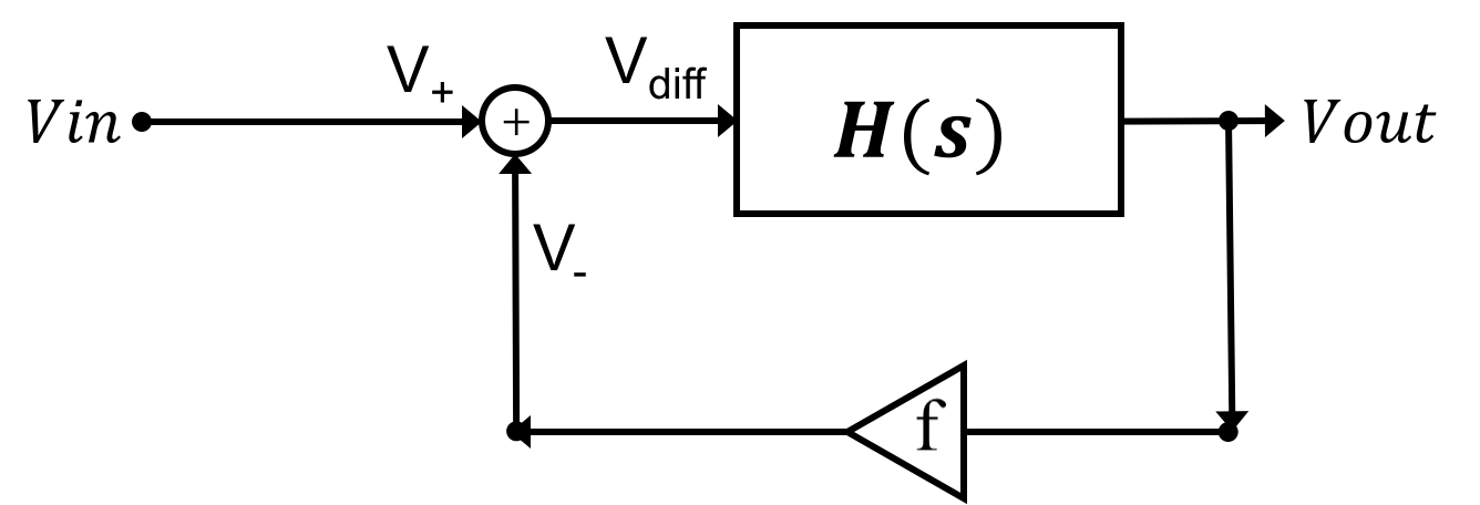
If we use what is usually referred to as non-inverting configuration, using resistors $R_{1}$ and $R_{2}$ to create the feedback network. This op-amp may be modeled using a feedback block diagram, with a 'forward-path' given by $H_{O P A M P} (s)$ and a 'feedback path' scaled by a factor $f$ .

This is not our usual tracking configuration, because the output is scaled by $f$ before comparing to the input, but this form is more natural when describing operational amplifier circuits. To analyze this case, we know that based on how the circuit elements are connected,

V_{+} = V_{i n}, V_{-} = f V_{o u t}

where

f

is LESS than one, and is determined by the resistor divider network.

The operational amplifier's output voltage, $V_{o u t},$ is determined by the product of its transfer function and the differential input voltage,

V_{o u t} = H_{O P A M P} (s) (V_{+} - V_{-}),

as is also shown in the block diagram above.

Combining,

V_{o u t} = H_{O P A M P} (s) (V_{i n} - f V_{o u t}),

resulting in a variant of Black's formula,

V_{o u t} = \frac{H_{O P A M P} (s)}{1 + f H_{O P A M P} (s)} V_{i n} .

where we have put the

s

back in the the equation to remind ourselves that we have a tranfer function with a frequency response. Note that

V_{o u t} \approx \frac{1}{f} V_{i n} .

when

| H_{O P A M P} (s) | >> 1

In the following examples, we we generate state-space models of op-amp circuits, in order to gain a better understanding of the relationship between state-space and the classical transfer function approach to control.

A low-gain op-amp example.

Consider the non-inverting amplifier using an op-amp as in the circuit below.

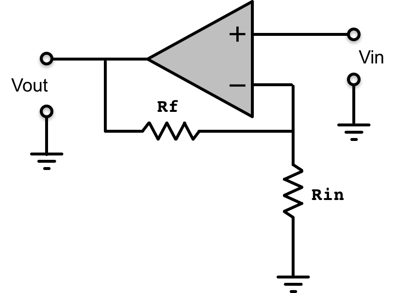
In the non-inverting op-amp circuit, with primary input, $v_{i n} (t)$ , and observed output, $v_{o u t} (t)$ , the closed-loop gain steady-state gain is

Closed loop gain = \frac{v_{o u t_{s s}}}{v_{i n_{s s}}} \approx 1 + \frac{R_{f}}{R_{i n}},

where we say "approximately" because the formula is only exact if the op-amp has infinite open-loop gain.

When we represent the non-inverting amplifier op-amp circuit using block diagrams, we use Laplace transforms to convert dynamics into transfer functions, and organize the feedback structure by separating the open loop gain stage from the subtraction stage. That is, we introduce

V_{+} = V_{i n},

V_{d i f f} = V_{+} - V_{-},

and

V_{o u t} = H (s) V_{d i f f},

as in the diagram below.

As an example, suppose $R_{f} = R_{i n}$ , then

1 + \frac{R_{f}}{R_{i n}} = \frac{R_{i n} + R_{f}}{R_{i n}} = 2,

and

f

, as in the above diagram, is given by

f = \frac{V_{-}}{V_{o u t}} = \frac{R_{i n}}{R_{i n} + R_{f}} = \frac{1}{2} .

If we have an ideal op-amp, then the non-inverting amplifier gain, $\frac{V_{o u t}}{V_{i n}}$ , will be equal to two. If we have a lousy op-amp, one with a steady-state gain of only 20, then the noninverting gain will be less than two. In particular, if the op-amp's transfer function, $H (s)$ , is given by

H (s) = \frac{V_{o u t}}{V_{d i f f}} = \frac{20}{s + 1},

then the closed-loop transfer function,

G (s)

, is given by

G (s) = \frac{V_{o u t}}{V_{i n}} = \frac{H (s)}{1 + f H (s)} = \frac{20}{s + 11} .

To determine the steady-state closed-loop gain, we evaluate

G (s)

s = 0

. For this case, the gain is

\frac{20}{11} = 1.8182

, significantly below the ideal case closed-loop gain of two.

By adding a resistor divider between $v_{i n}$ and $v_{+}$ , we could convert the approximate gain-of-two amplifier into an exact gain-of-one amplifier, but to do so, we would need to know the op-amp's exact transfer function (at least in steady-state). Such a strategy for designing a gain-of-one amplifier might not be particularly practical, but examining the strategy using a state-space approach will help clarify the roles of the matrices and vectors involved, and provide a concrete example of the often-confusing role of $K_{r}$ .

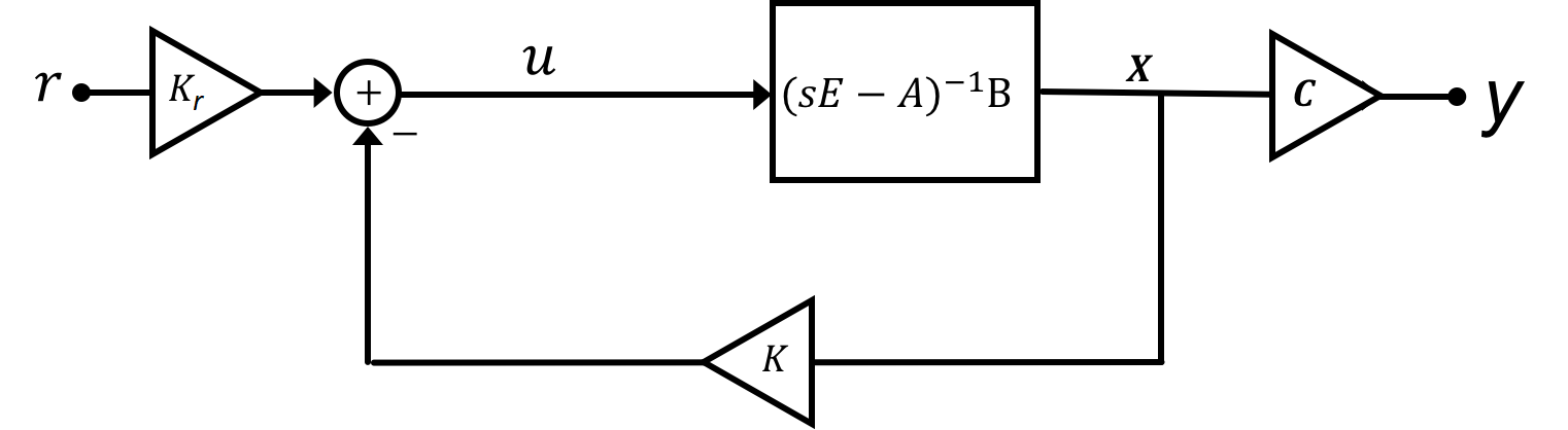
The generic State-Space Feedback System.

We can also describe the non-inverting amplifier circuit using a state-space model. The generic form of the state-space model using $E$ , $A,$ $B,$ and $C$ matrices is

E \frac{d}{d t} x = A x (t) + B u (t)

and

y (t) = C x (t),

or after Laplace transformation,

s E X (s) = A X (s) + B U (s)

and

Y (s) = C X (s) .

Reorganizing the transformed state-space model to more easily recognize the transfer function from the "plant" input, $U (s)$ , (distinct from the primary input $r (t)$ ) to the state, $X (s)$ , we get

X (s) = {(s E - A)}^{- 1} B U (s)

and

Y (s) = C X (s) .

Applying state feedback to the state-space system yields the block diagram below, where

K

is the state feedback gain and

K_{r}

is the scaling of the primary input,

r

State-space for Op-amps

How do we connect the block diagram for the op-amp to the block diagram for the state-space system? Let us consider a specific example, and suppose that the operational amplifier's open loop gain is given by

H (s) = \frac{1000}{s + 2}

and that

R_{f} = 3 R_{i n} .

If we write the differential equation for

v_{o u t} (t)

in terms of

v_{d i f f} (t)

\frac{d}{d t} v_{o u t} (t) + 2 v_{o u t} (t) = 1000 v_{d i f f} (t),

where

v_{d i f f} (t) = v_{+} (t) - v_{-} (t),

v_{+} (t) = v_{i n} (t),

and for the given resistor ratio,

v_{-} (t) = 0.25 v_{o u t} (t) .

To construct a state-space representation of this closed-loop op-amp circuit, suppose we choose to associate the state-space

u

with the op-amp voltage

v_{d i f f}

, then what are the state-space matrices?

For this op-amp example, all the associated state-space matrices are $1 \times 1$ (scalars), so we need only determine those scalar values. And in this case, we have NOT computed a $K_{r}$ to ensure unity steady-state gain. Instead, we are stuck with the $K_{r}$ that models the circuit. In fact, since $v_{+} = v_{i n}$ , $K_{r} = 1$ in this case. Also, we can assume that the observed output, $y$ , is equal to $v_{o u t}$ , so $C = 1$ .

The remaining matrices can then be determined by matching the generic state-space model with the op-amp circuit, please determine $E$ , $A$ , $B$ , and $K$ to complete the model. Note, since the matrices are $1 x 1$ in this case (scalars), give your answers as scalar numbers (For example, use $1$ and NOT $[1]$ or $[[1]]$ ).

Focusing On Kr

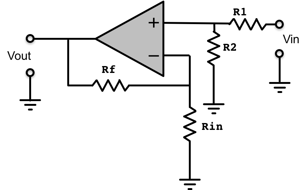
When we modeled the non-inverting amplifier circuit, $K_{r}$ had to be equal to one because $v_{+} = v_{i n}$ . But suppose we insert a resistor divider between $v_{i n}$ and $v_{+}$ , as in the diagram below.

We can use the divider to scale $v_{i n}$ and thereby change $K_{r}$ . Suppose we want to select a $K_{r}$ so that the closed-loop transfer function from input to output,

\frac{V_{o u t} (s)}{V_{i n} (s)} = C {(s E - (A - B K))}^{- 1} B K_{r}

is exactly one in steady state. At

s = 0

(for steady-state),

\frac{V_{o u t_{s s}}}{V_{i n_{s s}}} = - C {(A - B K)}^{- 1} B K_{r} = 1,

K_{r} = - \frac{1}{C {(A - B K)}^{- 1} B},

where we can use fraction notation since $K_{r}$ is a scalar.

The non-inverting op-amp circuit with $R_{f} = 3 R_{i n}$ implies the circuit was designed to have a steady-state gain of four, but by changing $K_{r}$ , we can achieve other steady-state gains, including EXACTLY unity. And since we can pick $R_{1}$ and $R_{2}$ in the above circuit to set $K_{r}$ , without altering $E$ , $A$ , $B$ , and $C$ , the values for the divider resistors are easily computed.

What is the EXACT value of $K_{r} = \frac{R_{2}}{R_{1} + R_{2}}$ so that the steady-state gain is EXACTLY one ( $K_{r}$ is approximately, but NOT EXACTLY, 0.25)!

R2/(R1+R2) =

What is the value of $K_{r}$ so that the steady-state gain is EXACTLY FOUR ( $K_{r}$ is almost, but NOT EXACTLY, 1)!

K_{r}

Check Yourself 1:

Can you implement a $K_{r}$ to get a steady state gain of EXACTLY four using a resistor divider on the input (No, do you see why)?

And what about the Pole?

When $K = 0.25$ , where is the pole of the closed-loop op-amp system?

pole =

If we made $K = 10$ , where is the pole of the closed-loop op-amp system? And for $K = 10$ , what value of $K_{r}$ will give us a steady-state closed-loop gain of EXACTLY one?

pole for K=10

K_{r}

at K=10

So, if we use a feedback gain of $10$ , meaning $V_{-} = 10 V_{o u t}$ , the above op-amp model suggests we can make the closed-loop pole far more negative, and therefore get step responses that are much faster. Though, to maintain a steady-state closed-loop gain of one, we will also have to scale the primary input, $v_{+} \approx 10 v_{i n}$ , or $K_{r} \approx 10$ . If we want a gain-of-one non-inverting amplifier to be ten times faster, we need two extra gain-of-ten amplifiers, hardly a practical trade-off. And if the op-amp's transfer function is more complicated, stability issues will also interfere (see the next example).

Check Yourself 2:

When we implement state feedback using microcontroller, we sense the states and then compute $u = K_{r} r - K x$ where $x$ is the sensed state and $r$ is the primary input. For example, $r$ could be the desired propeller arm angle, the elements of the vector $x$ could be the sensed angle, the sensed rotation rate, and the sensed propeller speed. The gains we multiply each of these sensed states by are much larger than one, but we do not even think about it. When we use a microcontroller to perform state feedback, we do not need an extra amplifiers whenever we want to scale a state by more than one. This simple observation is a big part of why the proliferation of inexpensive microcontrollers has dramatically increased the popularity of state-space controllers.

Three-Pole Op-amp Example in State-Space

Suppose the op-amp has an open-loop gain with the transfer function

\frac{V_{o u t} (s)}{V_{d i f f} (s)} = H (s) = (\frac{200}{s + 200}) (\frac{20}{s + 20}) (\frac{1000}{s + 2}) .

For the non-inverting amplifier configuration, what is the smallest integer value for

G_{i d e a l} = \frac{R_{f} + R_{i n}}{R_{i n}}

(the formula for the closed-loop gain in the IDEAL op-amp case) such that the system has a phase margin of

45

degrees, and when using those resistor values, what is the real part of the least stable pole and what is the actual closed-loop steady-state gain.

Lowest Gideal for 45 degrees phase =

Real part of least stable pole

Actual Steady-State Gain

We can model this more complicated op-amp in state-space, and a simple way to derive the state-space model is to introduce a few auxillary variables. We define

V_{3} (s) = \frac{1000}{s + 2} V_{d i f f} (s),

and

V_{2} (s) = \frac{20}{s + 20} V_{3} (s) .

Then

V_{o u t} (s)

is given by

V_{o u t} (s) = \frac{200}{s + 200} V_{2} (s) = (\frac{200}{s + 200}) (\frac{20}{s + 20}) V_{3} (s) = (\frac{200}{s + 200}) (\frac{20}{s + 20}) (\frac{1000}{s + 2}) V_{d i f f} (s) .

We can then write a series of differential equations,

\frac{d}{d t} v_{o u t} (t) = - 200 v_{o u t} (t) + 200 v_{2} (t)

\frac{d}{d t} v_{2} (t) = - 20 v_{2} (t) + 20 v_{3} (t)

\frac{d}{d t} v_{3} (t) = - 2 v_{3} (t) + 1000 v_{d i f f} (t) .

What are the state-space matrices for our three-pole op-amp model, assuming $x_{1} = v_{o u t}$ , $x_{2} = v_{2}$ and $x_{3} = v_{3}$ , and that we assign $u = v_{d i f f}$ and $y = v_{o u t}$ . Enter the $E$ , $A$ $B$ , and $C$ matrices below for the state space representation, (Remember to use Python form, so if $C$ is $[\begin{matrix} 1 & 15 \end{matrix}]$ , you should enter [[1,15]], and for a column vector, like $B$ , you should enter [[1],[15]].)

Check Yourself 3:

Why are the poles of the open-loop state-space system equal to the diagonals of the $A$ matrix? The poles of the open-loop system are the eigenvalues of $E^{- 1} A = A$ , since $E$ is the identity matrix. And since $A$ is triangular, its eigenvalues are its diagonal entries.

The Three Feedback Gains

For the non-inverting amplifier op-amp circuit, you determined the smallest integer value of $G_{i d e a l} = \frac{R_{f} + R_{i n}}{R_{i n}}$ so the amplifier would have a phase margin of $45$ degrees. Note that $G_{i d e a l}$ would be the closed-loop gain if the op-amp had been ideal, and in terms of $G$ (shorthand for $G_{i d e a l})$ , what is an expression for the ratio

\frac{V_{o u t_{s s}}}{V_{-_{s s}}} ?

Steady-State ratio Vout/V- =

The state-space model derived above can describe a non-inverting amplifier with ideal-op-amp closed-loop gain of $G$ , provided feedback gains are chosen appropriately. Assuming $G$ is still the smallest integer such that the closed-loop system has $45$ degrees of phase margin, what are the feedback gains $K_{1}$ , $K_{2}$ and $K_{3}$ for the state-space model of that non-inverting amplifier? And, what is the closed-loop system matrix, $A-BK$ .

A-BK

Notice the location of the non-zero value associated with the one nonzero component of $K$ . Does the change in one location of $A-BK$ cause a change in all the eigenvalues, or only one?

How many eigenvalues of A-BK are different from the eigenvalues of A?

Check Yourself 4:

Notice that the matrix $A-BK$ is not triangular, thanks to the fact that $(A - B K)_{3, 1} \neq 0$ . Therefore, the poles are no longer equal to the matrix diagonals.

With the above gains, what value of $K_{r}$ will give us a steady-state closed-loop gain of EXACTLY one?

K_{r}

If we can feedback a weighted combination of all three states, we can achieve far faster response times. Using Matlab's place command, find values for $K_{1}$ , $K_{2}$ and $K_{3}$ so that the poles of the closed-loop state-space system are $- 100$ , $- 110$ and $- 120$ . Additionally find the value of $K_{r}$ so that the steady-state gain is exactly one.

K_{r}

And what is the associated $A-BK$ ?

A-BK

Notice that it was not necessary to use very large gains to produce a dramatic improvement in performance. The performance was achieved by observing all the states in the system, and then acting on that collection of information. With classical control, the feedback was based on a single state (the output in this case), and the results were much poorer.

A quick trick of zero value for E

Suppose the open-loop transfer function for the op-amp gain had a zero, that is, suppose

\frac{V_{o u t} (s)}{V_{d i f f} (s)} = H (s) = (\frac{200}{s + 200}) (\frac{5 s + 20}{s + 20}) (\frac{1000}{s + 2}) .

Could you update the state-space system above to include the zero by only changing

E

? And if so, what would that change be?

We have used matlab's place command to determine the gains needed to place the closed-loop poles in specified locations. But to use the place command, the system has to be converted to "normal form",

\frac{d}{d t} x = A_{n} x (t) + B_{n} u (t),

or equivalently, $E_{n}$ matrix has to be the identity. What are $A_{n}$ and $B_{n}$ for our three-state system?

An=

Bn=

Find values for $K_{1}$ , $K_{2}$ and $K_{3}$ so that the poles of this new closed-loop state-space system are $- 100$ , $- 110$ and $- 120$ , and find the value of $K_{r}$ so that the steady-state gain is exactly one.

K_{r}

Could you have guessed how the $K$ 's would change after including a single zero in the transfer function? We could not.