State-Space One- and Two-Propeller-Arm Models

The questions below are due on Friday November 26, 2021; 10:00:00 AM.
 

Relating Arm Angle to Motor-Related Force

 

 

 

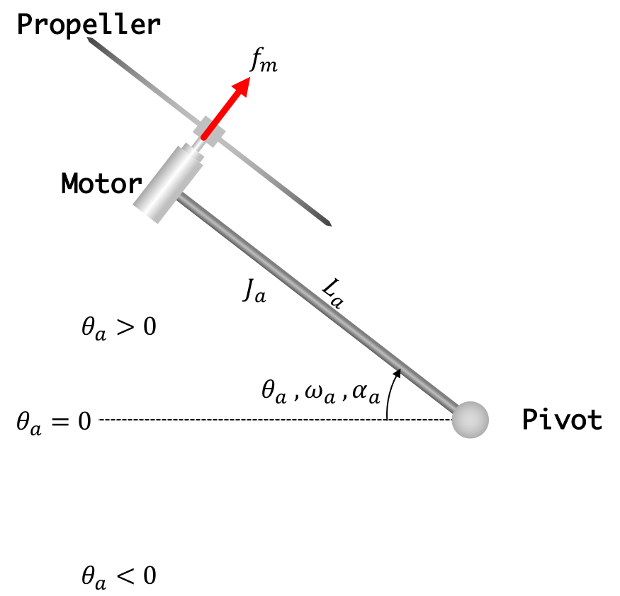
The angle of our propeller arm, \theta_a(t), is related to its angular velocity, \omega_a(t), through differentiation,

And in turn, the angular velocity of the arm, \omega_a(t), is related to arm angular acceleration through differentiation,

The arm's angular acceleration is equal to the torque on the arm \tau_a, divided by the arm's moment of inertia, J_a,

Since the chopstick has so little mass compared to the motor at the end of the arm, the moment of inertial for the arm is given by where L_a is the arm length and M_m is the mass of the motor.

There are two sources of torque on the arm, both of which act on the end of the arm. There is the upward thrust generated by the spinning propeller, and the downward gravity force acting on the mass of the motor. Since both forces act at the end of the arm, the torque on arm is equal to the product of arm length and net force in the direction of arm rotation,

where f_n is the net rotation-directed force.

The above relations can be combined to relate arm rotational velocity to the motor-related net force as

Linearizing the Motor Force-Speed Relation

The thrust force generated by a spinning propeller, f_m, is proportional to the square of the propeller rotation speed (which is also the speed of the motor, \omega_m). That is,

where K_{t0} is a propeller-specific thrust coefficient.

The thrust is a nonlinear function of motor speed, and we will need to linearize the relation about some nominal speed if we want to generate a linear state-space model. When we were controlling the arm angle with a PD or PID controller, we adjusted the nominal motor speed (using a direct term) so that the nominal arm position was nearly horizontal, or \theta_a \approx 0. Consider using that same nominal motor speed, which we will denote \omega_{m0}, to linearize the thrust-speed relation in a linear state space model.

When the arm is horizontal, the upward thrust generated by the spinning propeller exactly cancels downward gravity force. That is,

where g is the acceleration due to gravity, and M_m g is the gravity force acting on the motor.

Taylor-expanding the thrust-speed relation about \omega_{m0} yields

where \Delta\omega_m(t) \equiv \omega_m(t) - \omega_{m0} is the perturbed motor speed.

If we define f_n as the net force on a nearly-horizontal arm, then f_n = 0 if the motor speed is exactly \omega_{m0}, and f_n is proportional to the perturbation from nominal motor speed, as in

where linearized thrust coefficient, K_t, is given by. Note, we have assumed that for small perturbations from horizontal, the gravity force still cancels the nominal thrust, even though the cancellation is exact only when the arm angle is precisely zero. For small deviations from horizontal, the cancellation remains nearly perfect, do you see why?

Combining with the result of the previous section, we get a relation between arm angular acceleration and the perturbation in motor speed,

Note that in deriving the above relation, we invoked the nearly horizontal assumption multiple times.

The Motor-Speed Drive-Voltage Relation

The motor driving the propeller can be modeled as the series combination of a resistor, R_m, modeling the motor coil resistance, an inductor, L_m, modeling the motor coil inductance, and v_{emf}, a speed-dependent voltage source modeling the electromotive force generated by the coil spinning in a magnetic field. The current through the motor, i_m, can be related to the drive voltage, v_{pwm}, as shown in the schematic below. Note that the schematic also includes a series resistor, R_s,, which you can see on the controller PC Board (labeled R250). We use a (\frac{1}{4} \Omega) sense resistor.

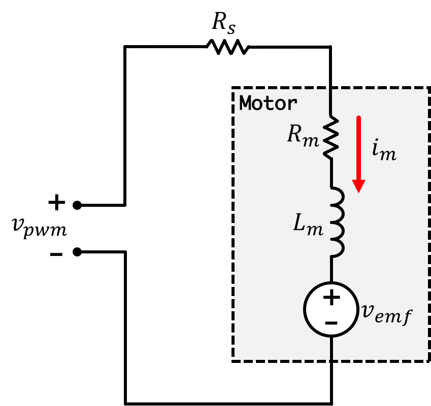
From the circuit,

but we can simplify this relation. The propeller motor inductance is so small,and the millisecond time scales relevant for controlling the arm are so long, that compared to \left(R_m+R_s\right) i_m(t) and v_{emf}(t), resulting in the simplified circuit below.

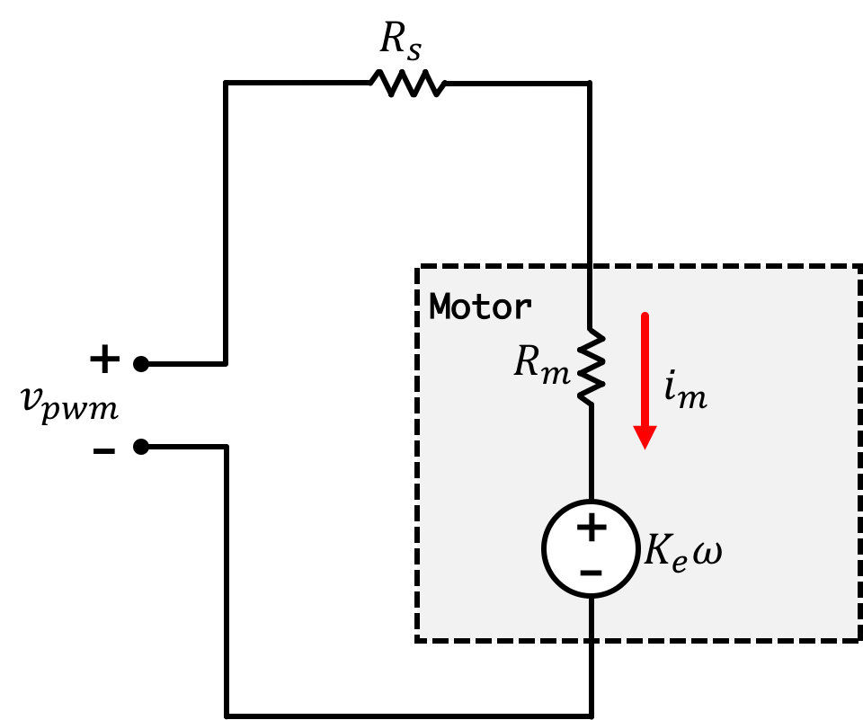
The motor back-EMF, v_{emf}, is proportional to the motor speed, \omega_m, as in

where K_e is the back-EMF constant for the motor.

By discarding the effect of propeller motor inductance, and using the above linearizations, we get an approximate relation between drive voltage and motor speed,

which can be rearranged as

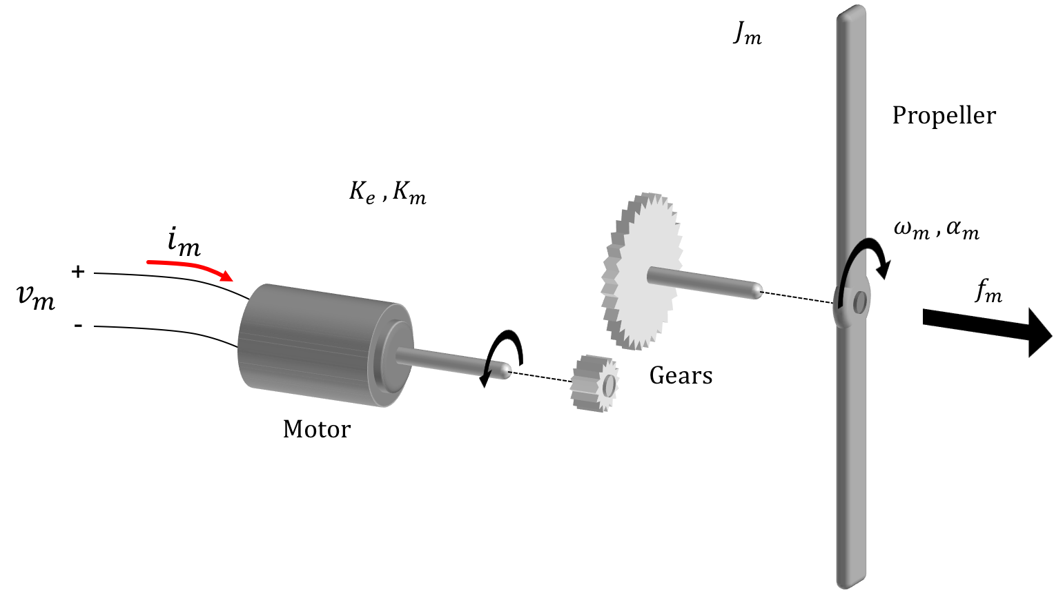
The motor torque \tau_m is proportional to motor current,

where K_m is the torque coefficient. The motor torque is equal to the product of motor acceleration, \alpha_m, and the motor-propeller moment of inertial, J_m,

Combining the current-voltage relation, the torque-current relation, and the acceleration-torque relation yeilds

We can include speed-dependent linear friction to the model by adding a friction force that reduces acceleration. If we denote K_f as a linear friction coefficient, we get:

and recalling that v_{emf} = K_e\omega_m, we can formulate the relation entirely in terms of v_{emf},

Matrix Construction

We've now filled in three equations which we can use to construct our state space matrices:

and
and

We know that v_{emf}(t) = K_e \omega_m (t) , and since \Delta\omega_m(t) \equiv \omega_m(t) - \omega_{m0} , we define \Delta v_{emf} as

Since the equation relating v_{emf} to v_{pwm} is linear, it follows that

Given \Delta v_{pwm}(t) \equiv v_{pwm}(t) - v_{pwm_0} , how will you determine v_{pwm_0}? You will need to understand this for lab!!!!!!

Using arm angle, arm angular velocity and perturbation in back-EMF, \Delta v_{emf}, as the three state variables, we have a linearized state-space system,

and also

It is important to remember which matrices above correspond to our state space setup:

Constants

It wouldn't be bad to start sticking numbers to some of the constants we've been using in our derivations and modeling.

• J_m = 3\times 10^{-6} N\cdot m (modeled as flat beam)
• K_e=K_m\approx0.5\times 10^{-3} V\cdot\text{rad}^{-1}\cdot s
• J_a = 4.5 \times 10^{-4} N\cdot m modeled as solid rod and point mass
• R_m=1 \Omega
• R_s=1 \Omega
• L_a=0.15 m

Adding Friction

Starting with the derived \textbf{A} matrix above representing our plant we can label the individual elements in it as follows:

\textbf{A} = \begin{bmatrix}a_{11} & a_{12} & a_{13}\\ a_{21} & a_{22} & a_{23}\\ a_{31} & a_{32} & a_{33} \end{bmatrix}

If we wanted to implement a rotational friction/drag coefficient on the arm, what term would we modify?

a_{11}

a_{12}

a_{13}

a_{21}

a_{22}

a_{23}

a_{31}

a_{32}

a_{33}

Loading...

Drag on the Propeller

With your propeller running with no feedback (just a low constant fixed voltage on the motor), if you were to quickly move the arm up or down (using your hand) you should notice (via the tone of the motor) that the motor speed is varying because of the forcing of more or less air through the propeller (varying the drag on the prop). How could we implement this phenomenon in our state space model?

Starting with the 3 \times 3 matrix \textbf{A} above, which represents our arm model, denote the matrix elements using the usual labeling,

\textbf{A} = \begin{bmatrix}a_{11} & a_{12} & a_{13}\\ a_{21} & a_{22} & a_{23}\\ a_{31} & a_{32} & a_{33} \end{bmatrix}.

If we wanted to add in a term capturing the phenomenon what term would we modify?

a_{11}

a_{12}

a_{13}

a_{21}

a_{22}

a_{23}

a_{31}

a_{32}

a_{33}

Loading...

Drag Value

How would drag modify the element of the \textbf{A} matrix you selected?

In what way would the presence of drag modify the element of the \textbf{A} from the previous question?

Increase its value

Decrease its value

Loading...

Our propeller arm system has a plant that can be described by the matrices derived above, and since E is the identity matrix, the eigenvalues of \textbf{A} are the poles or the natural frequencies of the plant. We will feed back a weighted combination of states to control the plant, as shown in the diagram below.

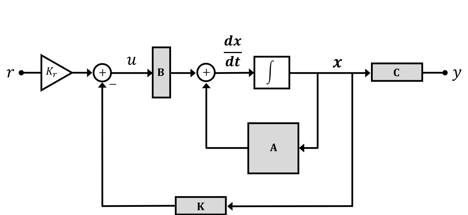
In the above diagram, E is assumed to be the identity, y is the output (the arm angle in our case), u is the input to the plant (v_{pwm} for the arm example), and r is the input to the feedback-controlled system (\theta_d, the desired arm angle). The state-feedback weights, or gains, are represented by \textbf{K}, a matrix with as many rows as inputs to the system, and as many columns as states in the plant.

This week, our approach to chosing the feedback gains is to adjust them to make the poles of the closed-loop system as stable as possible.

Proportional Gain

Starting with

\textbf{K} = \begin{bmatrix}K_1 & K_2 & K_3\end{bmatrix}=\begin{bmatrix}0 & 0 & 0\end{bmatrix}

If we wanted to implement proportional only control on the arm angle, what term would we adjust and how would we do it?

Make K_1 positive

Make K_2 positive

Make K_3 positive

Make K_1 negative

Make K_2 negative

Make K_3 negative

Loading...

Derivative Gain

When carrying out Proportional + Derivative Control (a PD controller), a gain K_d is applied to the derivative of the error signal. To implement PD control in a state-feedback framework applied to arm angle control, which values of the \textbf{K} matrix must be adjusted, and how?

Starting with

\textbf{K} = \begin{bmatrix}K_1 & K_2 & K_3\end{bmatrix}=\begin{bmatrix}0 & 0 & 0\end{bmatrix}

If we wanted to implement proportional+Derivative control on the arm angle, what terms would we adjust and how would we do it?

If we wanted to implement proportional+Derivative control on the arm angle, what term would we adjust and how would we do it? (assume we've already made the change specified in the previous question)

Make K_1 positive

Make K_2 positive

Make K_3 positive

Make K_1 negative

Make K_2 negative

Make K_3 negative

Loading...

Input (or Pre-Compensator) Gain

You may have noticed in the diagram earlier in the page there is a K_r term. This is sometimes referred to as precompensator gain, or just input gain. The reason for the gain is to scale the closed-loop input so that the closed-loop output settles to a desired steady-state. In the case of a tracking feedback systems (in which the closed-loop output should track the primary input r), an expression for K_r is easily derived.

Consider a standard state-space system with state feedback, as in

\textbf{E}\frac{d\textbf{x}}{dt} = \textbf{Ax} + \textbf{B}u,

y = \textbf{Cx},

and

u = K_r r - \textbf{K}\textbf{x},

where u is the input to the system being controlled, and r is the primary input to the closed-loop system.

Since we are considering a tracking system, a good controller should insure that the output y tracks the primary input r, and as a reminder, we will relabel r as the desired output, or y_d,

r \equiv y_d.

If the feedback system is stable, and y_d settles to a constant value denoted y_{d_\infty}, then the system will settle in to a steady-state. That is, the time derivative of the states will eventually go to zero,

\frac{d\textbf{x}}{dt} \to 0,

and the states and output will settle to limiting values denoted by the subscript \infty. That is, as t \to {\infty},

\textbf{x} \to \textbf{x}_{\infty},

and

\textbf{y} \to \textbf{y}_{\infty}.

Combining the controller (with relabeled primary input) with the state-space system description, and then evaluating the combination at steady-state,

\textbf{E}\cdot 0 = \textbf{Ax}_{\infty} + \textbf{B} \left(K_r y_d{_{\infty}} - \textbf{K}\textbf{x}\right)

and

y_{\infty} = \textbf{Cx}_{\infty}.

Shuffling the terms and then solving for \textbf{x}_{\infty},

\textbf{x}_{\infty} = -\left(\textbf{A}-\textbf{BK}\right)^{-1}\textbf{B} K_r y_d{_{\infty}},

which can be multiplied by \textbf{C} to generate the primary input to output (in steady-state) relation

y_{\infty} = -\textbf{C}\left(\textbf{A}-\textbf{BK}\right)^{-1}\textbf{B}K_r y_{d_{\infty}}.

Since input and output are both scalars, their ratio,

\frac{y_{\infty}}{y_d{_{\infty}}} = -\textbf{C}\left(\textbf{A}-\textbf{BK}\right)^{-1}\textbf{B}K_r,

should be equal to one since we are considering a tracking feedback system.

For the input/output ratio to be one,

1 = -\textbf{C}\left(\textbf{A}-\textbf{BK}\right)^{-1}\textbf{B}K_r,

which can be solved for K_r, yielding

K_r = -\left(\textbf{C}\left(\textbf{A}-\textbf{BK}\right)^{-1}\textbf{B}\right)^{-1}.

The above expression is a relation between the vector of state-feedback gains, \textbf{K}, and the precompensator gain, K_r. If one determines the state-feedback gains to achieve a particular dynamic performance, then one can adjust K_r to ensure perfect steady-state match. BUT, that match is perfect ONLY IF the state-space model is exact.

Input Gain associated with Proportional Control

In order to implement proportional control (a P controller), a gain K_p is applied to the error signal. If we want to implement the equivalent of proportional control using state feedback as in the block diagram above, would we need to modify K_r?

Yes

No

Loading...

Input Gain associated with Derivative Control

In order to implement proportional + derivative control (a PD controller), a gain K_p is applied to the error signal and a gain K_d is applied to its derivative. If we implement the equivalent of PD control using state feedback as in the block diagram above, will we need to update K_r if we only change K_d and NOT K_p?

Yes

No

Loading...

Adding a second propeller

This question is intended to give you a little more practice with generating state-space models (and manipulating them computationally), and we will need the two-propeller model when we do the observer lab. The answers to this prelab question will be checked during the observer/learned model lab because we are asking you to create a matlab model, and then check that your model makes sense. Such a question is too open-ended for us to evaluate your understanding entirely automatically, but we want to make sure you understand your model.

It is important to remember which matrices above correspond to our state space setup:

\textbf{E} = \begin{bmatrix} 1 & 0 & 0\\ 0 & J_a & 0 \\ 0 & 0 & J_m \end{bmatrix}

\textbf{A} = \begin{bmatrix} 0 & 1 & 0\\ 0 & 0 & \frac{K_tL_a}{K_e} \\ 0 & 0 & -\left(\frac{K_mK_e}{\left(R_m+R_s\right)}+K_f\right) \end{bmatrix}

\textbf{B} = \begin{bmatrix}0 \\ 0 \\ \frac{K_m K_e}{\left(R_m+R_s\right)} \end{bmatrix}

\textbf{C} = \begin{bmatrix} 1&0 & 0\end{bmatrix}

Double the Props, Double the Fun?

Suppose we want to add a second propeller, as in the figure below, how will we update the state-space model so we can design the controller? How many states does the system have? How do the equations change?

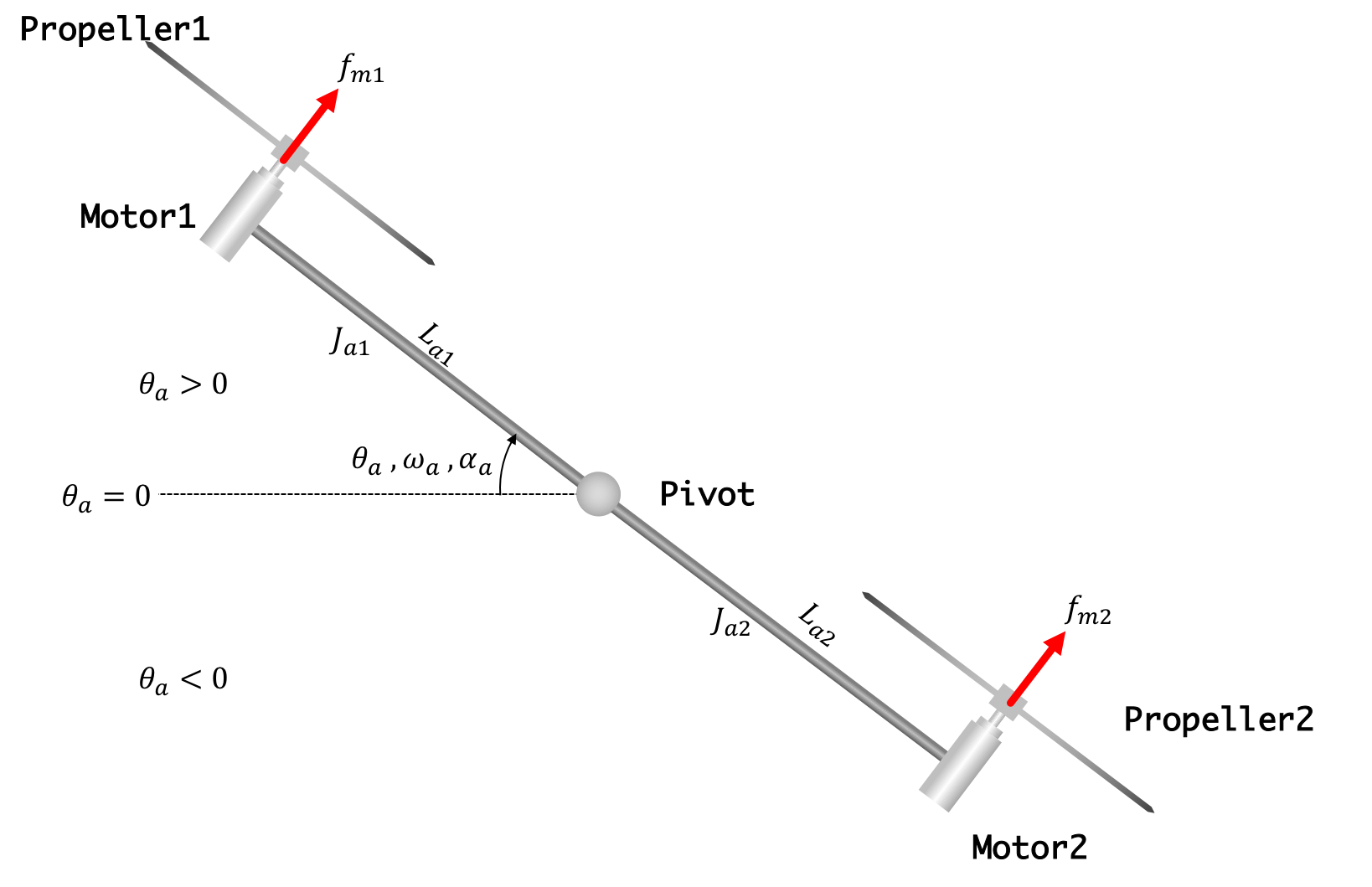
If we assume the entire arm is rigid, and the two motors are approximately identical in their characteristics, and make a few other approximations (see the derivation in the prelab if interested), then the moment of inertia for the two-prop arm is given by

J_a = \frac{1}{3} d_{rod} L_{a1}^3 + m_{prop}L_{a1}^2+\frac{1}{3}d_{rod} L_{a2}^3 + m_{prop}L_{a2}^2

where m_{prop} is the propeller+motor mass, d_{rod} is the density of the rods (the chopsticks in our setup, about 14 grams/meter) and L_{a1} and L_{a2} are the lengths shown in the figure above.

Linearization Questions and thoughts

In our motor thrust derivation, there is a big leap made concerning the linearization. We said that the thrust from the motor f_m is proportional to the square of the propeller speed \omega_m times a thrust coefficient K_{t0}:

f_m(t) = K_{t0}\omega_m^2(t)

To generate a linear system for the single propeller case, we Taylor-expanded the thrust-speed relationship about a nominal propeller speed, \omega_{m0}. We can perform a similar linearization for each propeller in the two-propeller case, and for motor one we get

f_{m1}(t) \approx 2K_{t0}\omega_{m10}\left(\omega_{m1}(t)-\omega_{m10}\right) +K_{t0}\omega_{m10}^2,

where f_{m1}(t) and \omega_{m10} are the thrust force and nominal propeller speed respectively for motor1. Similarly for motor 2 we get

f_{m2}(t) \approx 2K_{t0}\omega_{m20}\left(\omega_{m2}(t)-\omega_{m20}\right) +K_{t0}\omega_{m20}^2,

where f_{m1}(t) and \omega_{m10} are the thrust force and nominal propeller speed respectively for motor2.

Since positive thrust from motor1 rotates the arm clockwise (and increases the arm angle) but postive thrust from motor2 rotates the arm counter-clockwise (and decreases the arm angle), the two-prop-arm angular acceleration is proportional to the difference in propeller thrusts, as in

\frac{d\omega_a(t)}{dt} = \frac{L_{a1}f_{m1}(t) - L_{a2}f_{m2}(t)}{J_a}.

If we linearize both propeller thrust-speed relationships about the same speed, that is if

\omega_{m10} = \omega_{m20} = \omega_{m0},

and if the axis of rotation is equidistant between the two propellers, that is if

L_{a1} = L_{a2} = L_{a},

then we have some very fortuitous cancellations, and

\frac{d\omega_a(t)}{dt} =\frac{L_{a} K_t}{J_a} \left( \Delta \omega_{m1}(t) - \Delta \omega_{m2}(t) \right),

where \Delta \omega_{m1}(t) = \omega_{m1}(t)-\omega_{m0} and \Delta \omega_{m2}(t) = \omega_{m2}(t)-\omega_{m0}.

The above cancellation suggests that setting \omega_{m0} to produce a gravity-balancing thrust is no longer necessary. Thinking physically, the system is already exactly balanced when the arm angle is zero, even when the two propeller thrusts are zero! So why not just set the direct term and the nominal backEMF to zero for the two propeller case?

Is it as simple as that? Not really. Below is the plot showing actual thrust (in Newtons) as a function of propeller speed \omega_m, and we can see that the relation is quadratic. Therefore, the value of K_t above depends on what we choose for nominal motor speed. In our single-prop model, we used a value for K_t based on assuming a nominal motor speed of \omega_{m0} = 300\text{ rad}\cdot\text{s}^{-1}, resulting in a K_t= 1.78\times 10^{-3} N\cdot\text{rad}^{-1}\cdot \text{s}, but if we decided to make the nominal motor speed zero, we should get a very different K_t.

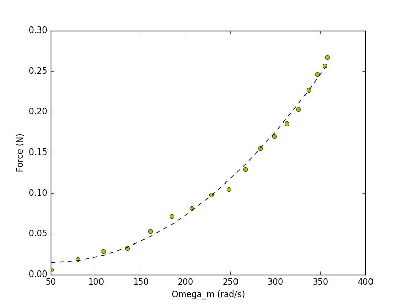
We fit an equation to the above plot of thrust versus motor speed,

f(\omega_{m}) = 2.55\times 10^{-6}\omega_{m}^2 + 0.00025\omega_{m} +0.02035,

and to determine K_t for a particular \omega_{m0}, we will need to differentiate the above expression. For example for 300 \;\text{rad}\cdot\text{s}^{-1}, we'd find:

\frac{df}{d\omega_{m0}} = 5.10\times 10^{-6}\omega_{m0} + 0.00025

and evaluating at 300 \;\text{rad}\cdot\text{s}^{-1} we get 1.78\times 10^{-3}.

What (approximately) is K_t when \omega_{m0}\approx 100\text{ rad}\cdot\text{s}^{-1}?

Loading...

The value of K_t is not all that changes when we change the nominal propeller speed. How rapidly the motor responds to changing commands is also effected. The time constant for speed changes, which you measured in a previous lab, is heavily dependent on the nominal motor speed.

If we change our nominal speed (by an associated change in direct value, what other Teensy parameters should change?

Nothing

modify Back EMF offsets

Use PID control

Loading...

Create A Model

We want you to come in with a full-state space model of the two-propeller system, and we will make use of the model in few weeks. Use the list of constants below and the MATLAB script at the top of the lab as starting point, and generate a MATLAB state-space model that we can use to determine gains for the two prop system.

% Script to compute propeller system using pole placement.
close all
clear all

% Parameters
Ke = 5.5e-3;  % back-emf per radian/sec motor rotational velocity
Km = 5.5e-3;  % Torque per amp
Jm = 3e-6;  % Motor moment of inertia
La1 = 0.21;   % Arm length in meters (one)
La2 = 0.21;     %Arm length in meters (two)
Ja = 1/3*(0.014)*La1^3 + 0.016*La1^2 + 1/3*(0.014)*La2^3 + 0.016*La2^2
Rm = 1;      % Motor resistance
Rs = 1;      % Series resistance
Kf = 10e-6;  % Motor Friction
Kt = 1.8e-3; %Torque coefficient for arm (300 rad/s)

Quick Questions

Answer these quick questions about the matrices for our new two-propeller state-space model.

What should the dimensions of our new \textbf{A} matrix be?

2\times 2

3\times 3

4 \times 4

5\times 5

6\times 6

Loading...

What should the dimensions of our new \textbf{B} matrix be?

4\times 1

3\times 1

4 \times 2

3\times 2

5\times 1

5\times 2

Loading...

What should the dimensions of our new \textbf{C} matrix be?

1\times 2

1\times 3

1 \times 4

1\times 5

2\times 3

2\times 2

2\times 3

2\times 4

Loading...

What should the dimensions of our new \textbf{K} matrix be (when we calculate it?

1\times 2

1\times 3

1 \times 4

1\times 5

2\times 3

2\times 2

2\times 3

2\times 4

Loading...