Observers

The questions below are due on Tuesday December 07, 2021; 09:00:00 AM.
 

1) Limitations of Full-State Feedback

In the last few weeks we've discussed the benefits and some very basic techniques for designing state space controllers. So far this has generally involved:

• Coming up with a set of physical relationships that we can use to model the system in question

• Constructing a set of difference equations using those physical relationships

• Identifying system states, and then merging our difference equations into matrix-based equations of the form:

  • \textbf{x}[n+1] = \textbf{A}_d\textbf{x}[n] + \textbf{B}_du[n]
  • y[n] = \textbf{C}_d\textbf{x}[n] + \textbf{D}u[n]

• Taking the system's state vector \textbf{x} multiplying it by a gain vector \textbf{K}_d and using the output modify the input signal (via negative feedback)

• Use the desired natural frequency locations along with manual or computational methods to solve for appropriate \textbf{K}_d values, while keeping in mind that we keep the system's states and and command signal (input to \textbf{B}_d) at reasonable levels. This will often be an iterative process.

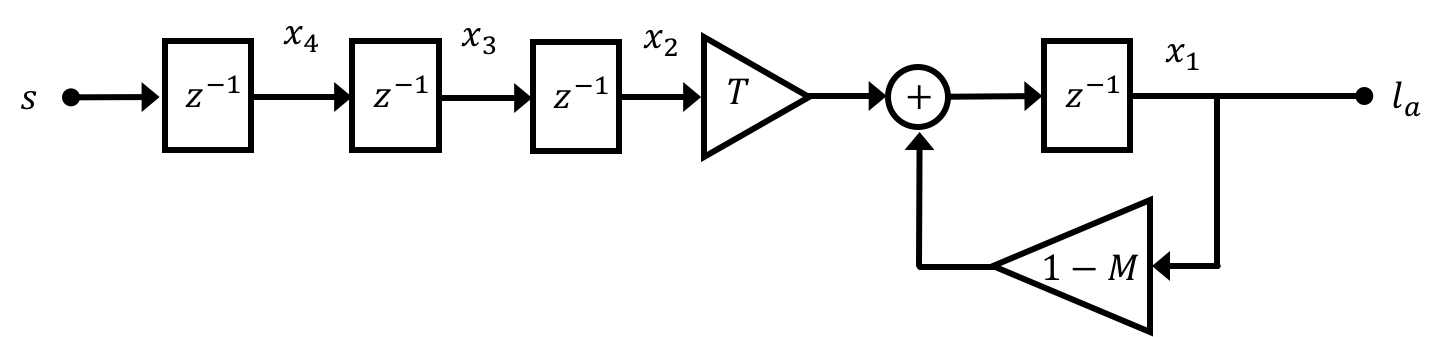
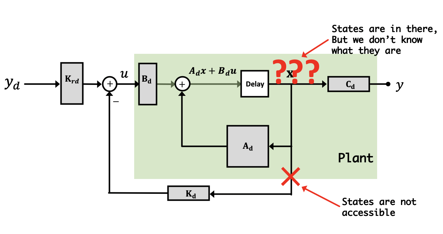
This can be a pretty reliable way of going about designing and controlling state space systems, however it is making one major assumption: that we have access to all of the system's states. To understand what is meant by this consider our anesthesia problem from last week. There are a number of states in this model, which can be thought of as modeling different biological membranes/barriers/transfers in the body (lung-to-blood, blood circulation, blood-to-brain, etc...). The "meaning" of these states could then be thought of as the current rate of anesthetic compound moving through those different barriers at different points in time:

Now if we pause and think about the amount of equipment and sensors needed to actually get at that information in real-time, you'll quickly recognize that full-state feedback as presented, while nice sounding would be way too invasive to properly implement on a person. In addition are questions about instrumentation...how would you even measure the transfer rate of anesthetic compound through the blood-brain barrier in real time? The answer is you wouldn't and this happens a lot in state space control. There are often numerous states in system models that we come up with that cannot, because of a lack of practicality (financially, physically, etc...), be measured. So while we might want the top system below, the bottom system is sometimes what we have to deal with. What do we do? The solution is Observers!

2) What's an Observer

2.1) Observers

An observer is model that we simulate of our system in real-time (so it will be done on the microcontroller at run-time). The observer is a state space system in its own right, so it has states and we'll want to avoid confusing them with the states of the real system. In order to distinguish its states (the simulated states) from the actual states of the real plant, we're going to denote them with a "hat" so that the observer's state vector will be \hat{\textbf{x}}[n]. Similarly we'll say the output of the observer is \hat{y} to distinguish it from the output of the actual plant y. As stated above, the observer is a full-on state space system so it can be described by its own set of state space equations like that shown below:

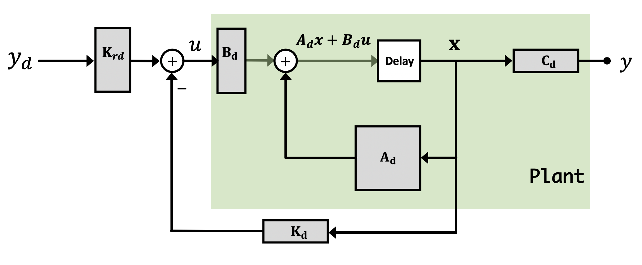
Now why are we doing this? Because the observer is a simulation, we have access to all "parts" of it, including the states. If we can make sure that our simulation accurately reflects the behavior of the real system, it probably means that the states of our simulated system are similar to what the actual states are. If this is so, we can use these simulated states to fill in for the "real" states that we cannot get access to from our real plant. We can multiply these estimated states by a gain vector \textbf{K}_d in just the same way as we were doing with our regular states from before. Diagramatically what we're doing is illustrated below:

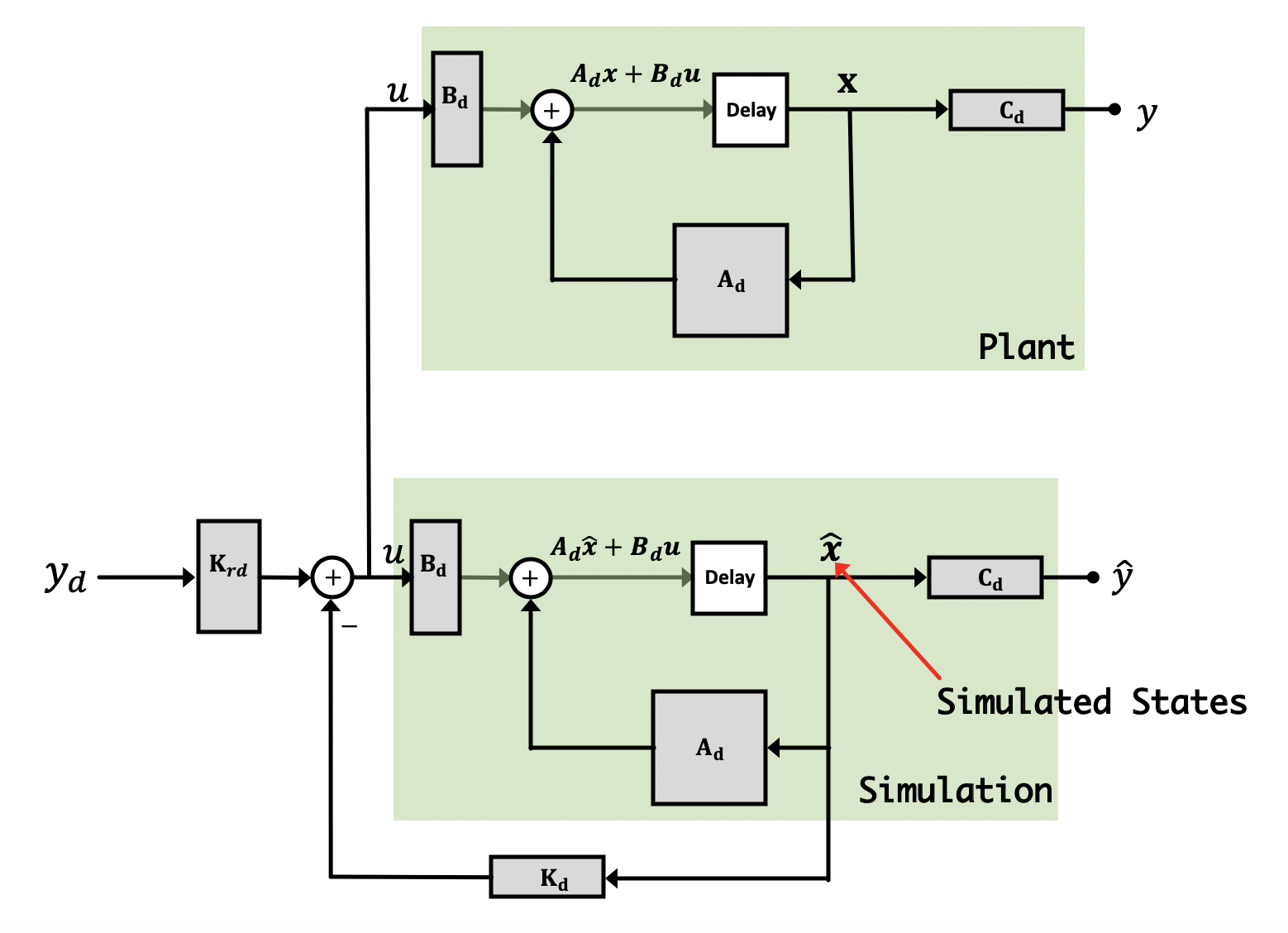
and this now implies that our system's primary state space equation (for the real states) is based on the following:

Of course, our goal is to have our estimated states track really well the real-life states so ideally we'll be able to say: \hat{\textbf{x}}[n] \approx \textbf{x}[n] at which point the above would simplify back to what we really want (effective full state feedback):

But is it really that simple? Unfortunately no, and we'll go over why in the following sections.

2.2) Moment to Reflect...

Now it is super important to remember/grasp/understand that there are two different "plants" in this combination of a physical and a virtual (observer) system. The physical plant exists and produces outputs that we can measure, it is the plant we are trying to control. The second plant is part of our observer and it is virtual. We are responsible for evolving the observer's state and computing its outputs, a process we often refer to as simulation in real time. Implementing an observer requires additional lines of code, and usually more computation. This is partly why we use a Teensy and not some slower Arduino Uno. While an Uno can control our propeller at the sample rate we've been running the Teensy, the additional arithmetic operations required to update the observer state on each iteration (on top of everything else) requires enough additional computation that the Arduino Uno can just not keep up with.

Using simulation alone to learn about observers can be confusing, because there is no difference between the physical plant and the virtual observer plant, everything is being simulated. The idea that one set of states are simulated as part of the control algorithm, and one set of states are simulated to act as a stand-in for the physical plant, is a subtlety easily missed when first learning this material. It is important to recognize that in MATLAB simulations, our simulation is simulating two things: The first is our real system, and the second is a simulation (our observer). When it comes time to deploy this on the levitating copter arm, the universe and Newtonian Physics will take care of "simulating" the first state space system (our physical one), and on our microcontroller we'll be left only needing to implement/simulate the observer version.

3) The Uncorrected Observer

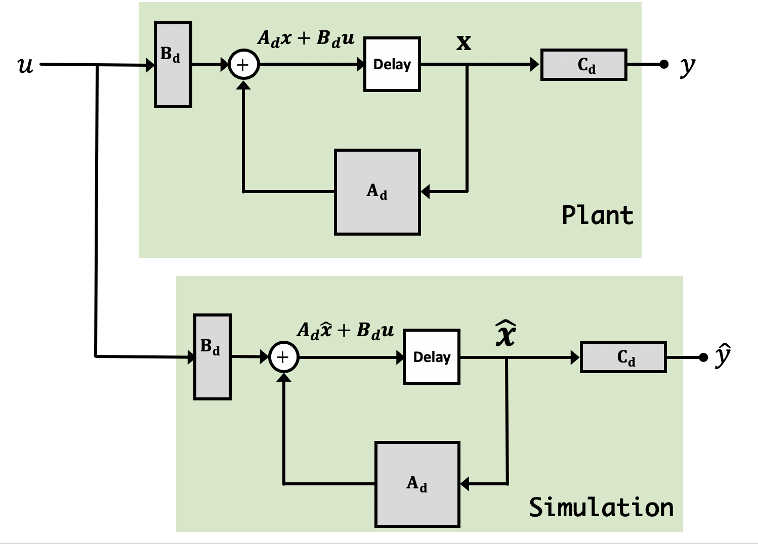
Consider a situation where we run an observer in parallel with our regular system in full-state feedback like shown below:

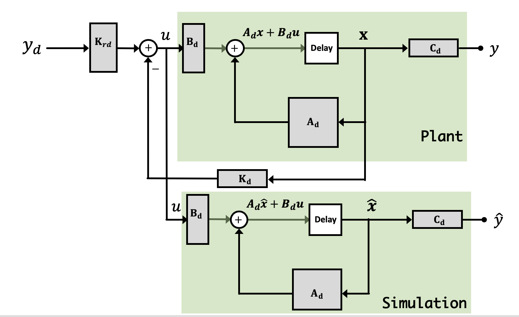
In this example, the physical plant is running with measured-state feedback, but in addition, we've added a simulation running in parallel to the real life system, and arranged that the input to the simulation is the same as the input to plant. That is, u for the plant is identical to u for the simulation.

3.1) Uncorrected Poles

What are some conclusions we can make about this "uncorrected" observer (that is, we do nothing to correct any errors between the simulated and actual states)? In particular, is the uncorrected observer guaranteed to be stable?

3.2) Uncorrected States and Inexact Observers

Consider the following simple plant with two states, x_1 and x_2,

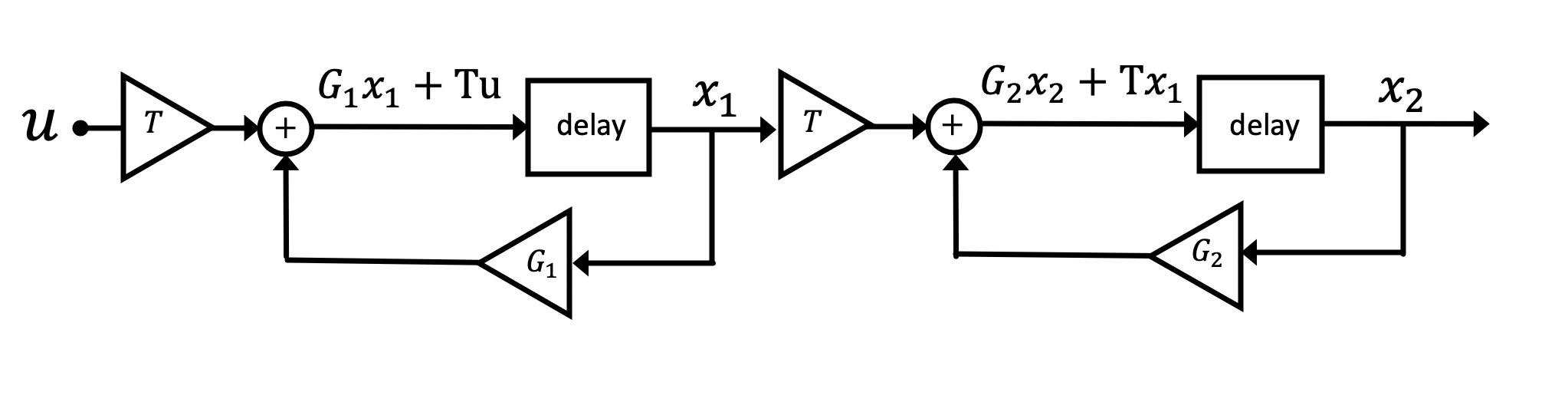
If we create a virtual plant, a copy that we evolve through simulation, we could refer to the state of actual plant as

and the state of the simulated plant, an uncorrected observer, as We could assume our virtual plant is an exact copy of the physical plant, or we could also assume our virtual plant is only approximate copy, so that G_1 and G_2 in the physical plant is not exactly equal to G_1 and G_2 in the virtual plant. How will the behavior of the uncorrected observer be affected?

To understand how an inexact observer with uncorrected states behaves, it is helpful to define a description of the differences between actual and virtual plants. We refer to the difference between the two plant states as the "uncorrected observer" state error, \textbf{e}, given by

Let us assume that for our two-state example, both the physical and simulation systems start at rest (all states are 0), and we apply a unit step to both systems, u[n] = 0,\;\; n \lt 0\;\;\;u[n] = 1\;\;n \ge 0.

First, lets assume that in our plant and in our observer, the values of G_1 and G_2 are 1, both have the same unit step input, and that both use a timestep T=1. After 10 seconds (10 time steps) what will error vector, that is \textbf{e}[10], be?

After 10 seconds (10 time steps) what will the values of our error vector be?

Now suppose the observer does not exactly match the physical system. Specifically, suppose that for the observer, G_1=G_2=1, and for the physical plant, G_1 = 0.95 and G_2 = 1, a relatively small mismatch, the observer is only 5\% different from the physical system. If we give both our plant and our observer a unit step input, after 10 seconds (when n=10) what will the values of our error vector be? Answer to three significant figures. Read the solution afterwards!

After 10 seconds (10 time steps) what will the values of our error vector be?

4) Feedback for Our Observer

As your experience must already make clear, our models are never perfect...we often ignore inconvenient forces, like gravity, and linearize highly nonlinear relations, like the one relating propeller thrust to motor back-EMF. Basically our model, while grounded in some of the physics, is not a good enough match to our physical system, so its simulated states will not track the actual states unless corrected. And the longer the simulation runs, the bigger this uncorrected observer error.

Since we use feedback to compensate for imperfections and disturbances when controlling our system, we should be able to use feedback to do the compensate for imperfections in our observer! That is, we can place the observer in a feedback system. But how? Like shown in the image below:

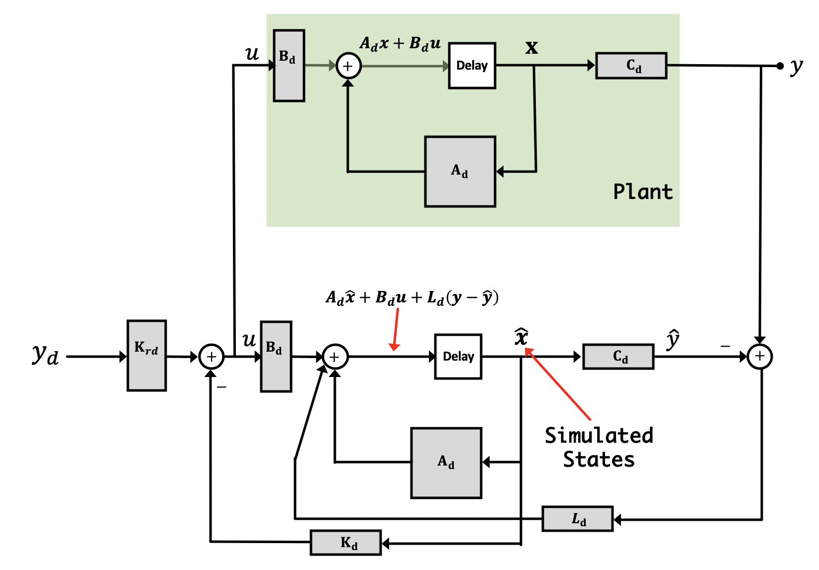
We're now going to create an output error signal we'll call e_y[n] which we'll define as:

We'll use this error signal, multiplied by a gain vector \textbf{L}_d to correct the system's states.

In state feedback, we adjust a row vector of state gains, \textbf{K}_d, so that the output output tracks a given input, y_d. In the observer, we're using output feedback, and we adjust a column vector of output gains, \textbf{L}_d, so that the estimated states track the physical states. This is as much a feedback problem as when we're controlling the system's output, and we'll want our observer to be able to converge quickly on the actual values so that we can use them in a timely manner to control the greater system. So, for example, we might choose \textbf{L}_d so that during a step response, the state estimate error decays twice as fast as the steady-state error. This is critical; if our observer's state estimates take too long to converge, they won't be accurate until it is too late to use them!

To analyze observer convergence, we return to the error vector \textbf{e} mentioned above,

Deriving state space expressions for the observer results in:

And then our actual plant state space expression would be:

Subtracting the expression for the estimated state, \hat{\textbf{x}}, from that of the actual state\textbf{x} we can come up with a state space expression for the error vector:

and if we remember that: ...we can then factor some stuff out so that it will be: or finally:

Now using the what we've learned about feedback and control in the last few weeks, this equation format should look very familiar. When placed into feedback like this using the difference of the two outputs (estimated and actual) as well as a feedback observer gain of \textbf{L}_d we can adjust the eigenvalues (natural frequencies) of the error signal, which means we can control how quickly our observer can correct its estimated state vector to match with the actual state vector!

If we think of the error vector and our original state vector as now as components of a much larger state space system (with state vector shape of 2\times m where m is the number of states) like that shown below and interesting characteristic will appear:

The new 2m \times 2m \textbf{A}_d matrix takes on the shape of a Block Upper Triangular Matrix which can be shown to have the following property:

This independence of the determinant means that the eigenvalues of the entire system will be the union of the eigenvalues of \textbf{A}_d-\textbf{B}_d\textbf{K}_d and the eigenvalues of \textbf{A}_d - \textbf{L}_d\textbf{C}_d! What this is saying is that the we can pick the values of our feedback gains \textbf{K}_d and our observer feedback gains \textbf{L}_d independently so we don't have to interweave their derivation. In fact, we can use similar tools to pick an \textbf{L}_d that gives us fast decay of observer state errors, as we use to pick a \textbf{K}_d that gives us fast step responses. But, there are differences in our objectives in the two cases. Mostly importantly, we want the state estimation error, \textbf{e}, to decay much faster than the tracking error, y-y_d.

Finally instead of having a hybrid state space expression with the error vector, we can instead write down our system with the m physical states and our m estimated states:

and

5) Picking our L

Using the place function to determine a \textbf{K}_d that places the closed-loop system poles (or closed-loop system natural frequencies), given by the eigenvalues of \textbf{A}_d - \textbf{B}_d * \textbf{K}_d , at chosen locations, we are assuming that our system is "controllable". The definition of controllable is covered precisely in more advanced control classes, but for our purposes, controllability is equivalent to being able to find a \textbf{K}_d that places the eigenvalues of \textbf{A}_d - \textbf{B}_d*\textbf{K}_d (the closed-loop poles) anywhere we choose.

Along with controllability a system has a dual property, "observability", which for our purposes, means that we can arbitrarily move the natural frequencies of a system observer around, and while we'll avoid the derivation here, we can also assume our systems have this property. Therefore, just like we had complete theoretical freedom in moving the eigenvalues (natural frequencies) of our plant around by manipulating \textbf{K}_d in the expression \textbf{A}_d-\textbf{B}_d\textbf{K}_d, we will be able to pick the \textbf{L}_d in the \textbf{A}_d - \textbf{L}_d\textbf{C}_d to place the observer poles anywhere we want.

The job of picking an \textbf{L}_d to place the poles of \textbf{A}_d - \textbf{L}_d\textbf{C}_d in desirable locations is similar to, but NOT exactly like the way we picked \textbf{K}_d. The shapes of \textbf{L}_d and \textbf{C}_d are different than the shapes of \textbf{K}_d and \textbf{B}_d , and they appear in a different order in \textbf{A}_d - \textbf{L}_d\textbf{C}_d than in \textbf{K}_d and \textbf{B}_d appear in \textbf{A}_d - \textbf{B}_d\textbf{K}_d.

A little linear algebra fixes the problem. To see this, first note that in general, the eigenvalues of a matrix are invariant under transposition. That is,

So if we transpose \textbf{A}_d - \textbf{L}_d\textbf{C}_d, its eigenvalues remain unchanged, Notice that \textbf{A}^T_d - \textbf{C}^T_d\textbf{L}^T_d is in exactly the same form as \textbf{A}_d - \textbf{B}_d\textbf{K}_d. So, we can place the eigenvalues of \textbf{A}_d - \textbf{L}_d\textbf{C}_d by using the place function, where inputs to place will be \textbf{A}^T_d, and \textbf{C}^T_d (these tranposed matrices have the same shape as the \textbf{A}_d and \textbf{B}_d matrices).

We will also need to transpose the vector returned by place . Note that \textbf{L}_d is m\times 1 matrix, so has the same dimensions as \textbf{B}_d, and its shape is the transpose of the shape of the 1 \times m matrix \textbf{K}_d.

5.1) Measurement Noise and Estimator Convergence.

When picking state gains, the \textbf{K}_d vector, mathematically we were nearly unrestricted in where we could place poles using place. We could not co-located multiple poles, for example, but other than that, we could place the poles anywhere. That was not as true with dlqr, even with R set to a very small number, because, for example, if one state was the derivative of the other, we could not drive them both to zero at the same rate. But whether we use 'place' or 'dlqr' to design the controller for a physical system, we had to ensure that

was within the drive capability of our controller. For example, on the propeller arm, the magnitude of u could be no larger than a few volts.

So what about the vector of estimator gains, \textbf{L}_d. Since the \textbf{L}_{d} \left( y - \hat{y} \right) only affects the observer system, a simulation, there are no physical limitations. So why don't we pick an \textbf{L}_{d} that gives us incredibly fast estimator convergence? Why not just use the 'place' command and place the natural frequencies very near zero? The answer is while we don't have to worry about state values being too high or our command signal being too large, we do need to worry about large values in \textbf{L}_d because they will amplify any output measurement noise. Because small natural frequencies/eigenvalues are generally associated with larger \textbf{L}_d values, this means that very fast responding observers will potentially cause trouble.

The rationale for this is the following: In looking at our estimator the \textbf{L}_d is applied to the

If we were to add in an additional signal w[n] representing a small amount of noise on the output, it would go where the output value y[n] is located (think of it as a noise signal "on top" of the output signal.

We can consequently adjust our error vector's \textbf{e} state space expression: and then: One way to accelerate the convergence of the state estimators is to pick an \textbf{L}_d that minimizes the largest magnitude eigenvalue of \left(\textbf{A}_d - \textbf{L}_d\textbf{C}_d\right). Generally, achieving a the smaller maximum eigenvalue requires an \textbf{L}_d with large magnitude entries, but that will magnify the impact of any output measurement noise.

The simplest setting in which to examine measurement noise is the steady-state case. We will denote the constanst steady-state noise as w_{ss}, though you can think of steady-state noise as a measurement offset error.

If w[n] = w_{ss} for all n, and if the eigenvalues of \textbf{A}_d - \textbf{L}_d\textbf{C}_d are all less than one in magnitude, then

has a steady-state. That is, and so Moving the error terms to the left hand side and then inverting, we get a relation between w_{ss} and \textbf{e}_{ss} in the form of a matrix inverse multiplied by the vector \textbf{L}_d w_{ss},

The \textbf{L}_d w_{ss} term in the above equation suggests that large magnitude values in \textbf{L}_d vector will amplify measurement noise, leading to very noisy state estimates. But \textbf{L}_d also appears in the matrix inverse multiplying \textbf{L}_d, so understanding the impact of large entries is not yet clear. We will look at the inverse matrix a bit more carefully below, but the complete answer requires a statistical analysis that is beyond the scope of this class, and leads to one of the most famous results in system theory, the Kalman filter.

If we chose \textbf{L}_d maximize the rate of state estimate convergence, or equivalently, to accelerate the decay of state estimation errors, we could try to minimize the maximum magnitude eigenvalue of \textbf{A}_d - \textbf{L}_d\textbf{C}_d. If that maximum is less than one, the estimation errors will decay, and the smaller the maximum, the faster the decay. We can relate these small eigenvalues to the eigenvalues of the above matrix inverse, to gain some insight into how it scales the noise. Using the spectral mapping theorem mentioned in the pre-labs, the eigenvalues of

are related to the eigenvalues of \textbf{A}_d -\textbf{L}_d\textbf{C}_d by If all the eigenvalues of \textbf{A}_d -\textbf{L}_d\textbf{C}_d are vanishingly small, then and therefore where If \textbf{L}_d is chosen so that state estimation converges extremely rapidly, so that then the steady-state noise in the state estimates will be equal to the steady-noise in the measurements, amplified by the entries in \textbf{L}_d.

The above result is less satisfying than it sounds, because picking \textbf{L}_d so that the eigenvalues of \textbf{A}_d - \textbf{L}_d\textbf{C}_d are nearly zero, will almost always require an \textbf{L}_d with huge entries, and the resulting magnification of the measurement noise will lead to very noisy state estimates. Instead, we could set the eigenvalues of \textbf{A}_d - \textbf{L}_d\textbf{C}_d just small enough to insure that the estimator error decays faster than the controller dynamics.

For example, suppose the controller poles, the eigenvalues of \textbf{A}_d - \textbf{B}_d\textbf{K}_d, are all greater than 0.95. Then setting the eigenvalues of \textbf{A}_d - \textbf{L}_d\textbf{C}_d to be less than 0.9 \approx 0.95^2, will result in estimator convergence nearly twice as fast as the controller dynamics. If the estimator system has eigenvalue magnitudes less than 0.9, then

The above bound on the eigenvalues of \left(\textbf{I}-(\textbf{A}_d - \textbf{L}_d\textbf{C}_d)\right)^{-1} indicates less than one would like. If all the eigenvalues of a matrix are equal (all being equal to 1, for example, as in the super-fast converging case), then the eigenvalue is a bound on the matrix. But if the eigenvalues are not all equal, one knows surprisingly little, because eigenvalues are the wrong tool to use. Instead, one must turn to singular values.

Consider the following example,

transposing both sides and multiplying by the original, The eigenvalues of the symmetric matrix \textbf{M}^T\textbf{M}, which are real and positive, are also the square of the singular values of \textbf{M},

The maximum singular value, \sigma_{max} can be used to bound the norm on \textbf{v},

where \textbf{v} and \textbf{w} are vectors and \textbf{M} is a matrix. Then the length norms (or l-2 norm, or eculidian, or...) are related by (removing all the squares), where is the maximum SINGULAR VALUE of \textbf{M}.

If we want to determine the impact of changes in \textbf{L}_d on the sensitivity of state estimation to measurement noise, then we will need to know the singular values of \left(\textbf{I}-\left(\textbf{A}_d - \textbf{L}_d\textbf{C}_d\right)\right)^{-1}. But, that is a topic for the next class in control. For now, we can just use simulation.

Singular values, Kalman filters,...so much more to learn.