Thermal Example

The questions below are due on Tuesday December 07, 2021; 09:00:00 AM.
 

This thermal problem makes use of the matlab script thermal.m.

As you have discovered, it can be very difficult to design a controller by first selecting candidate poles, and then using a program like place to determine the associated gains. The problem is that natural frequencies can have a complicated impact on trade-offs we care about, such as minimizing response time without exceeding equipment limits. What proved to be more effective is picking the state and input weights in a linear-quadratic regulation (LQR) scheme. In a previous postlab, we considered using LQR on a scalar discrete-time problem, mostly to gain insight into LQR. In this problem, we will try using LQR on a discrete-time system associated with temperature regulation.

A Temperature Control Example

Suppose you are designing the controller for a five-compartment heating system, as shown in the figure below. The pink compartment in the figure is the heater , whose temperature we assume can be set directly, so we denote it as the system input, u . The temperatures in the other four compartments, x_1, x_2, x_3, and x_4, are the system states. And since the compartments are placed contiguously, they are heated by pairwise bilateral thermal conduction, as diagrammed by the bi-directional red arrows in the figure. The equations above the red arrows follow from assuming that thermal conduction is proportional to compartment temperature differences, though we should note that the scale factor, g , is NOT a thermal conductivity. When we relate the rate of compartment temperature change to a g-scaled directional sum of compartment temperature differences, as in the equations below, we are implicitly assuming that the compartments are cubes, and that g is the thermal conductivity to specific-heat ratio.

Having encapsulated the physical details in g, the equations for the temperature change in one sample period, \Delta T, are not complicated. The change is equal to the product of the period length and the difference between the "flow" in from the left, and the "flow" out to the right. That is,

where \Delta T is the sample period in minutes and x_i is the temperature of the i^{th} compartment in centigrade degrees. For those more familiar with other temperature scales, recall that for centigrade, zero is the freezing point of water, 20 is a comfortable room temperature, and 100 is the water boiling point.

Controller Design and Equipment Constraints.

For this heating system, the control problem is to adjust the heater's temperature so that all four compartments achieve a desired temperature as quickly as possible, and then adjust the heater to maintain that temperature. But, this physical system has constraints. Allowing the heater to get too hot, even briefly, is dangerous. Very high heater temperatures could start a fire, or increase the frequency and severity of accidental burns. In addition, allowing compartment temperatures to exceed the target by more than a few degrees, even temporarily, may be problematic (particularly if the compartments are occupied).

The heating system constraints should not be dismissed as a problem-specific nuisance. Every real system has physical constraints, and addressing them is a central part of control system design. If fact, we started this section with a very specific physical example, rather than equations and derivations (but those are coming too), because the constraints are easily lost in the mathematics, as is the motivation for finding a design approach other than placing natural frequencies.

Determining the Gains.

We can formulate the temperature control problem as a single-input, single-output A,B,C,D state-space system,

where \textbf{x} = [x_1,x_2,x_3,x_4]^T , u is the heater temperature, and the A,B,C,D matrices can be found in the

In the matlab script, there is a line near the top,

poles = [0.5,0.5,0.5,0.5];

which sets the desired poles, or natural frequencies, for the feedback system. These natural frequencies are used by place to determine the feedback gains,

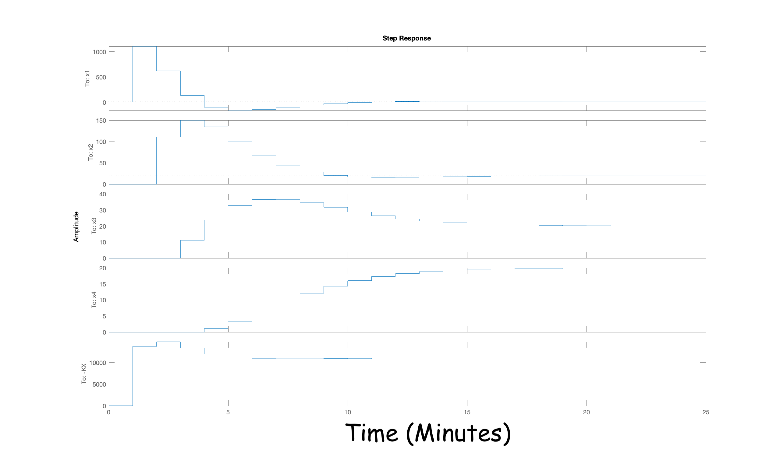
If you try running the matlab script as is, you should see something like the figure below. And if you examine the simulated compartment and heater temperatures, you should notice several important characteristics. First, the controller is fast, the compartments settle to room temperature in less than 15 minutes. But, you should also be alarmed by how that speed was achieved.
The maximum temperatures are thousands of degrees, and the heater has to get hotter than the surface of the sun!!. And it may seem a little anti-climactic, but notice that temperature of the heater also has to go negative, and refridgerate the compartments.

Clearly setting all the natural frequencies to 0.5 was too aggressive, but what should we do? Should we set all the natural frequencies to the same value, or should we chose several different values? And what values? In the next question, we will ask you to find natural frequency values so that place produces gains that give you controller performance that matches ours. The question is not graded, try it three times by editing the matlab script thermal.m (see the link at the top of the page), then look at our results and verify them in your code.

And before you start the next problem, please keep in mind our key point. It is very difficult to find the natural frequencies that gave a good result, Learn about LQR, another tool for determining controller gains.

For this problem, you will be determining the gains for a better controller for the four-compartment heating system, by using the natural frequency placement approach (more commonly referred to as pole-placement). Please answer the questions below by modifying the natural frequencies in the matlab script thermal.m (see the link at the top of the page). The code will do most of the mechanical work for you, and plot the simulation results for your designs.

You will be trying to pick natural frequencies that lead to a controller that minimizes the time for the compartments to settle to their final temperatures, while satisfying constraints associated with the physical system. The two constraints your solutions should always meet are:

1. The maximum temperature of the heater must be less than 60.
2. The maximum temperature in any compartment should not exceed 20.1 degrees (one tenth of a degree above the target).

Modify the natural frequency placement in the thermal.m file to set all the natural frequencies to approximately 0.99 (we have to offset them slightly for matlab's place command to work). That is, change

poles = [0.5,0.5,0.5,0.5];

to

poles = [0.99001,0.99002,0.99003,0.99004];

With all 0.99 natural frequencies, how many minutes does it take for all the compartment temperatures to be within one degree of their target temperature?

Can you find a set of natural frequencies that performs better than the results shown below (satisfies the constraints and settles to within one degree in less than 165 minutes)?

We found the following four:

[0.63,0.73,0.87,0.98]

Using OUR answer for the natural frequencies in the previous problem, and then use the matlab script to determine the associated gains for our set of natural frequencies. What were the related set of gains, to 2 digits of precision? Please note, this question is intended to help you verify that you understand the script.

K_1

K_2

K_3

K_4

Did you find natural frequencies for the heating system problem that were better than ours?

	Yes
	No