Week 2 Lab: PIDdling.
Please Log In for full access to the web site.
Note that this link will take you to an external site (https://shimmer.mit.edu) to authenticate, and then you will be redirected back to this page.
PID (Proportional, Integral, Derivative) controllers are ubiquitous in feedback systems, though for discrete-time systems, it would be more accurate to refer to such controllers as PSD (Proportional, Sum, Delta). An ad-hoc approach to designing a PSD controller is to select a proportional feedback gain, K_p, and then increase the gain of the Delta feedback, K_d, until the step response is sufficiently stable. Finally, add Sum feedback, with gain K_i, to eliminate any remaining steady-state error. We will start today's lab by implementing a PSD controller, to gain some insight into the role proportional, delta and summation feedback play in system performance. But we will also learn the limits of our intuition, and appreciate the need for a model that we can use to automate the search for better controller gains.
But if we can easily run experiments, even automate the running of those experiments, what is the value of an accurate LDE (linear difference equation) model? Well, with a model we can get far more information that just the result of a single input-output experiment. If we can compute the closed-loop system's natural frequencies as a function of PID controller gains, K_p, K_d, and K_i, we learn how the closed-loop system will response to a whole of range of inputs and disturbances. So for example, we could use the model to solve a minimax problem with respect to the magnitude of those natural frequencies. That is, we could let the computer search through millions of senarios, to find the gains that minimize the closed-loop system's maximum magnitude natural frequency. We would then be sure that resulting closed-loop system would be fast, and that any errors would decrease rapidly. But we digress. There is much to the story of data and models, some of it with connections to machine learning, and this issue will reemerge many times during the semester.
Back the matter of finding a good model. In last week's lab and postlab, we used a
If we add the dynamics that relate motor command to thrust, and further complicate the system by including the sum (integral) term in the controller, we will have a daunting analysis problem if we have to rely on the rather cumbersome procedure of shifting indices in difference equations. Instead, we will make judicious use of a key Z transform identity: that shifts in index correspond to multiplication by z^{-1}. We will use this identity to convert difference equations into rational functions in z, also known as transfer functions, and then use matlab's computational tools to manipulate these transfer functions.
To reduce steady-state errors, we can add an integral, or more precisely, a sum feedback term to our controller. Any persistent error, no matter how small, will cause the sum to grow steadily. When the sum term is large enough, it will cause an adjustment to the motor command, persumably an adjustment that eliminates the small error.
The motor command with the proportional, delta, and sum feedback can be described by the difference equations
YOU WILL HAVE TO IMPLEMENT THE SUM TERM IN THE TEENSY SKETCH!
Use the link at the top of this page to download the PID Teensy sketch (DO NOT the use the PD sketch fromlast week!!), and look at lines 454-456 (approximately) in the Teensy sketch. Notice that we have not implemented the sum term, but we have defined the Ki, errorSum and SumMax variables for you to use. Look for lines with comment FIX THIS!! and ensure that:
- Sum is computed correctly
- SumMax is set to a reasonable value, and
- Ki*errorSum is included in the motorCmd calculation on line 460.
Notice that we have defined a 'deltaTSecs' near the top of the Teensy Sketch, use it if you need the time interval. Do not use 'deltaT', as it is in the units of microseconds (one million times too large).
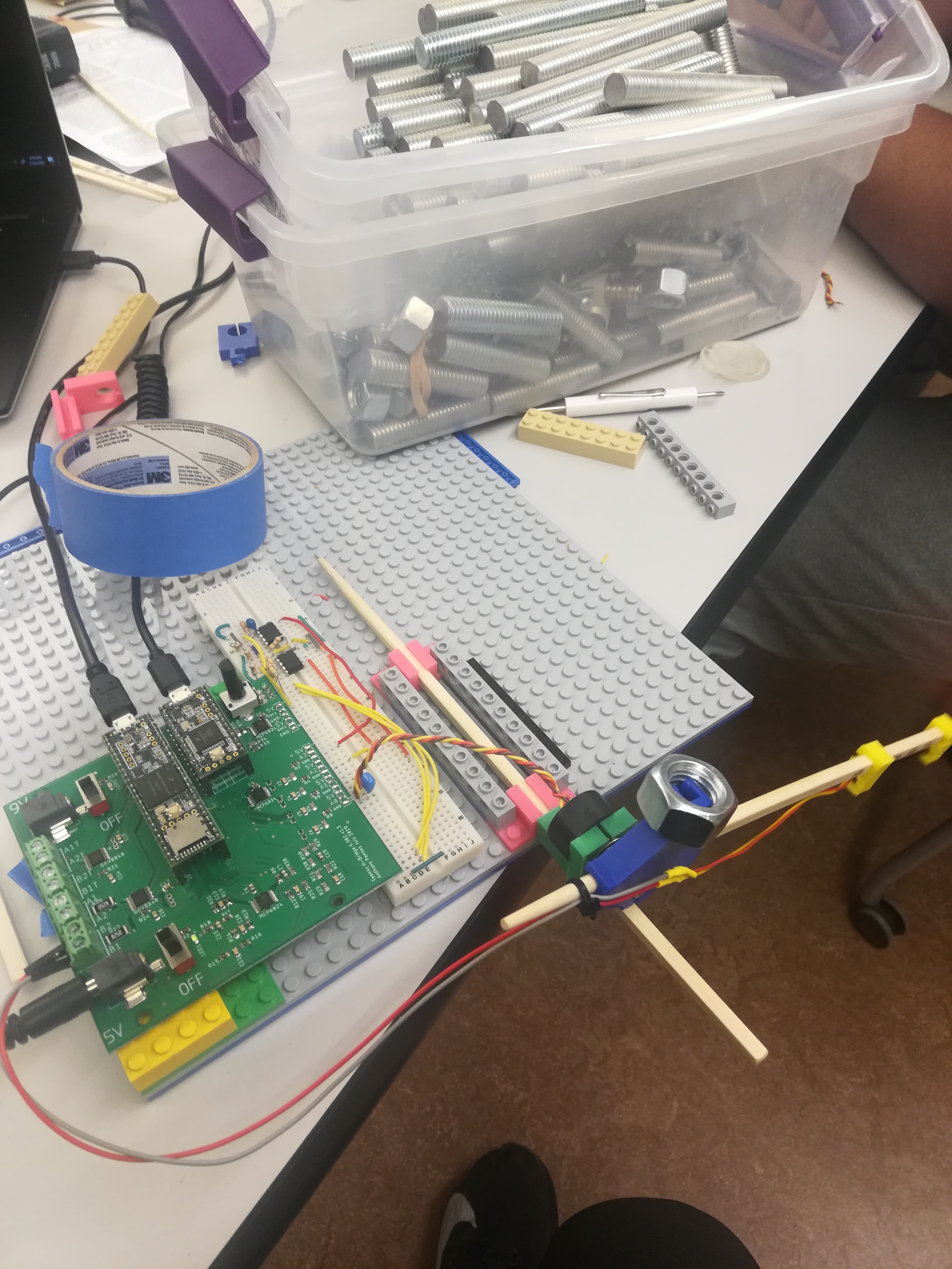
Connect your control laptop to the control Teensy and flash with the PID sketch, connect your monitor laptop to the monitor Teensy (the vertical Teensy), flash the monitor Teensy with USB_repeater sketch (same one as last week), start the server on your monitor laptop, open the gui (in Chrome or Firefox), click the reconnect button, and you should see the now familiar array of graphs and sliders. If you are having issues with your set up flying everywhere adding lego supports like in the image below
- Use the sliders to set Kp = 1, Kd = 0.3, and desiredAngle = 0.0. Then at the top of the PID sketch, recalibrate your angle sensor, and then adjust the value of cmdNominal so that the copter arm is almost exactly horizontal (and the angle error plot shows the error is nearly zero).
- Tip your entire setup upwards, and note what happens to the angle error.
 How to tilt setup
 - Set the desiredAngle slider to 0.1, causing the desired angle to toggle between positive and negative 0.1. Note the magnitude of the steady state error when the desired angle is 0.1 and -0.1.
- Be sure you added the Sum (also know as the integral) term to the Teensy code, as mentioned above.
- Try implementing the Kp and Kd values from the last week's lab and look at the steady state error.
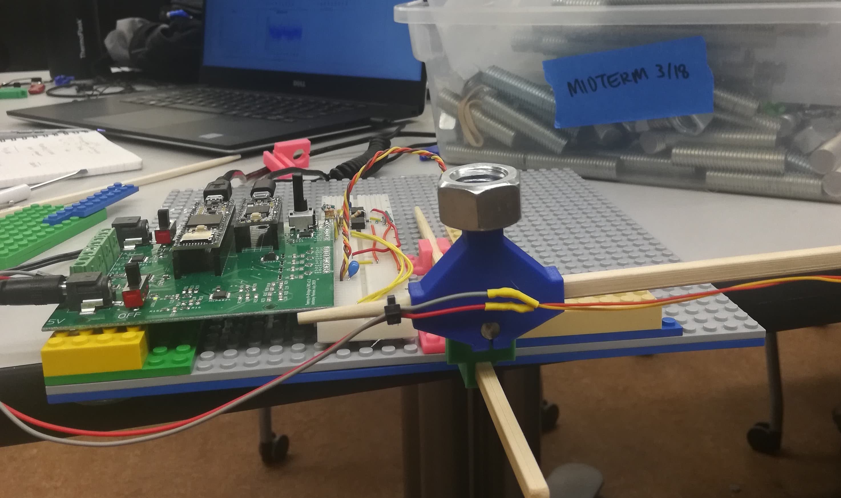
- Try some experiments: Add a nut as in the image below then slowly increase Ki, but watch out, the arm may fly up. Try with longer and shorter values for togglePeriod (between 1 and 5). What happens to the steady state error at 0.1 and -0.1?
- Try some experiments: set the 'cmdNominal' to zero at the top of the control sketch (don't forget to reflash), tip your setup, disturb the propeller by poking at it, etc. What are the consequences of adding sum feedback?
- With the Sum gain set to a moderate value (but with the system still stable) hold the arm down for several second. Let go of the arm and allow it to stabilize again. What happens? What role does SumMax play?
- Try to find a set of three gains that gives you good performance by trial and error. Be prepared to defend your notion of good.

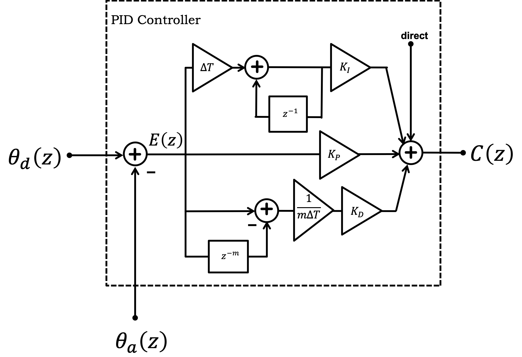
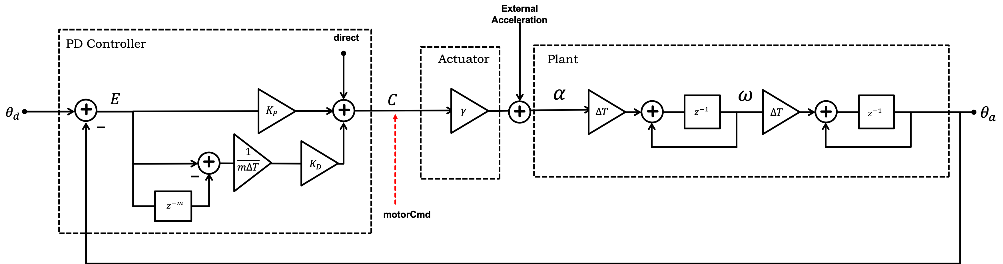
In the matlab script 'lab02.m' (see the link at the top of this lab), we used the Z-transforms to describe the PD-controlled copter arm model given in the diagram below.
In the matlab script linked at the top of the page, we created transfer functions for each subsection of the above model, though we just used a constant \gamma for the model of motor command to rotational acceleration. Note that we started by telling matlab that z was a transform variable,
>> z = tf([1 0], [1], -1); dt = 0.001;
and then created transfer functions using z. For example, we created 'hw2th', the transfer function from angular velocity to angle, using
>> hw2th = dt/(z-1)
Note that we entered the transfer function with only positive powers of z.
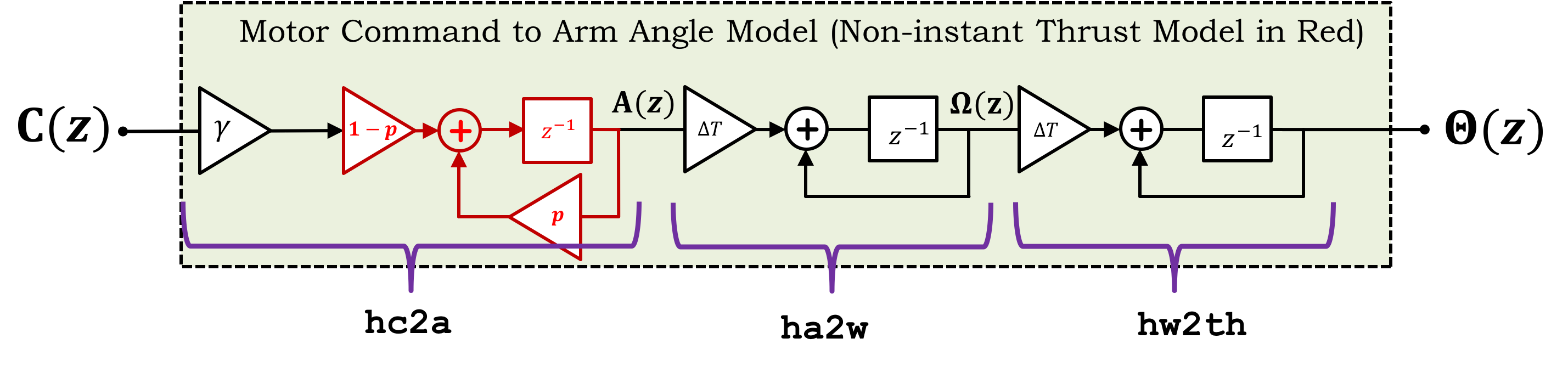
Last week, our assumption that rotational acceleration changes instantly with change in motor command, or equivalently, A(z) = \gamma C(z) where A(z) is the arm rotational acceleration in the figure above, or also equivalently, hc2a = \gamma. As you will see below, the transfer function relating acceleration and motor command should be the product of a single pole and \gamma, so that hc2a = \gamma \frac{1-p}{z-p}. You will be adding this to the matlab script, and examine how the poles (natural frequencies) change.
Note that there is also
- `ha2w`: the transfer function from acceleration to angular velocity,
- `hc2a`: the transfer function from command to acceleration without the pole,
- `Hc2th`: the complete open loop model without the pole (just the product of the others!!).
Try running the matlab script, and see that it plots step responses and displays closed-loop system natural frequencies (or poles).
As noted in the introduction, representing the relationship between the arm rotational acceleration and Teensy motor command with a simple proportionality constant is too inaccurate. While it is true that arm acceleration is related to the propeller thrust by a proportionality constant (the arm's moment of inertia), and if linearized about a nominal propeller speed, changes in thrust can be related to changes in propeller speed by a proportionality constant, but changes in propeller speed are not related to changes in motor command in such a simple way.
Propeller speed is accelerated or decelerated by changes in motor current, and motor current is a function of the motor command and the propeller speed (because of the backEMF). So if we represent the relationship between the motor command and the arm angular acceleration by the proportionality constant, \gamma, we ignore an important dynamic that has a significant effect on closed-loop stability. Instead, we will use a more accurate model for the thrust-command relationship, a product of \gamma and a first-order difference equation (see the block diagram below).
In order to determine a difference equation's coefficients empirically, you will use the 6302_FF_control sketch. You should download the sketch, set its cmdNominal value to the same one you used in the PID controller (so you are linearizing the systems about the same point).
When there is a step change in motor command, neither the propeller rotational velocity, nor the copter thrust, jump instantly to a new steady-state. Instead, they evolve in time, eventually settling to a new steady state. This is indicative of the presence of a non-negligible natural frequency(ies) or pole(s) in that part of the plant. If we model this evolution of rotational acceleration with a first-order difference equation, then we can augment our model of the copter-levitated arm, as shown in red in the arm block diagram above. And since rotational acceleration is proportional to thrust, and thrust is an algebriac function of propeller speed (although an admittedly nonlinear one), they have similar dynamics. So, we can estimate the parameters for a first-order difference equation model that relates motor command to rotational acceleration by examining the dynamic behavior relating motor command to propeller speed. Good thing we examined motor speed in Lab 0, it will come in handy now!
We will examine motor speed step responses using the feedforward Teensy sketch, and estimate the pole for a one-pole (or one natural frequency, or first-order difference equation) model. The form we use for the complete model will force a steady-state scaling equal to \gamma to complete motor-command to angular-acceleration model.
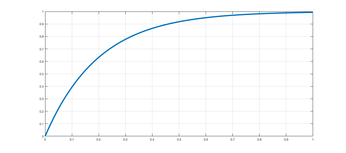
Before examining motor speed step responses, let us take a moment to review how to extract a first-order difference equation model from a continuous time waveform. Suppose we wish to model the above step response, in which w(t) is plotted versus t, using a first-order difference equation of the form
If \Delta T = 0.001, what are good values for p and B? In estimating the values for p and B, take particular note of the above waveform's steady-state, and the time when the waveform reaches half of that steady-state. For example, suppose w is defined by a difference equation
Estimating a time constant for the propeller spin up.
Determining the parameters of a first-order difference equation model of the relation between the motor command and the propeller acceleration, as in
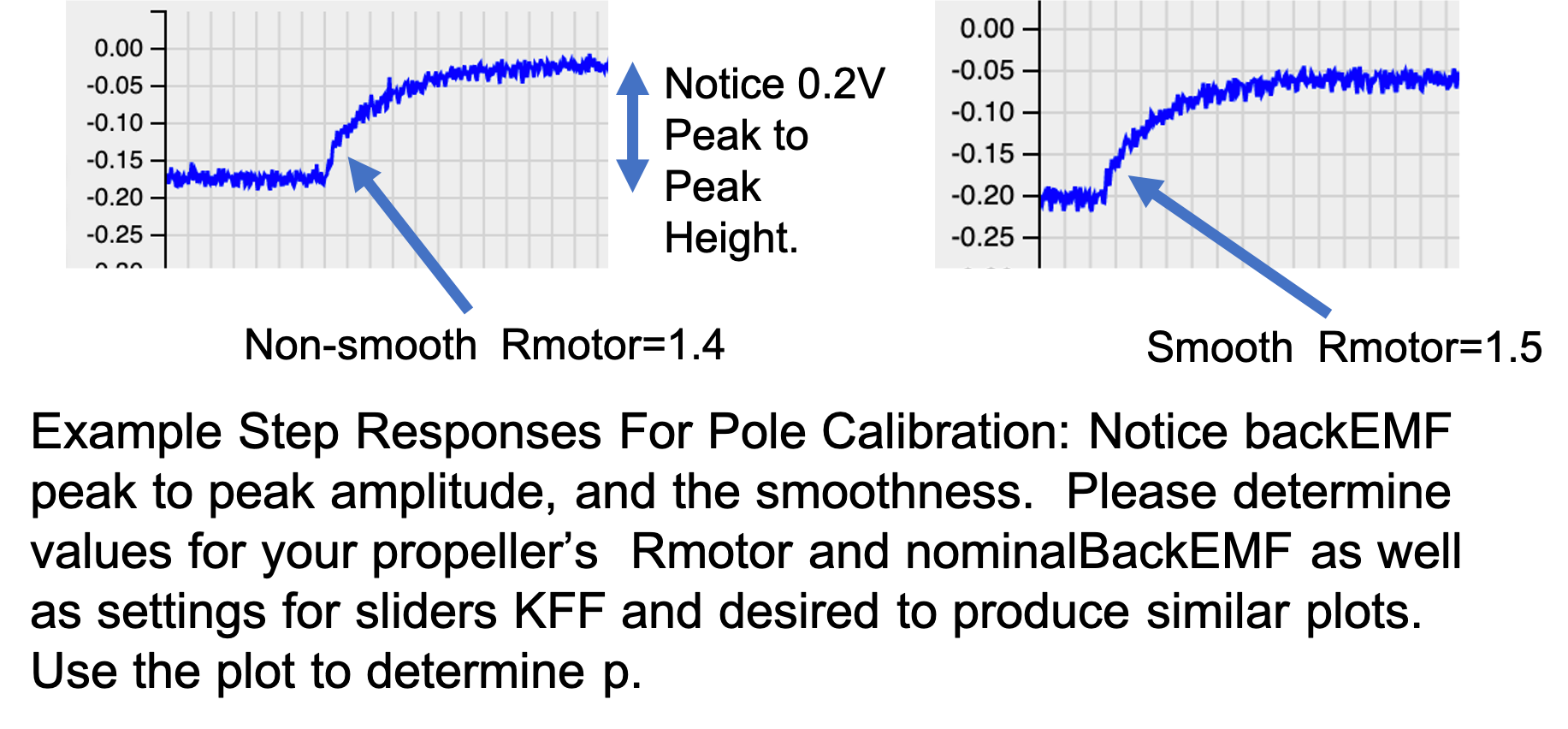
To determine the pole, p, we can use a setup similar to the speed control Lab00, to make step changes in the motor command, and monitor the backEMF. The feedforward Teensy sketch at the top of this lab, 6302_FF_control, can be used to generate the steps and plot the backEMF (look at the last 40 lines or so to get an idea of how motorcmd is calculated).
When running 6302_FF_control, you should set cmdNominal to the value needed to set the arm horizontal in the PID controller (with Ki = 0). Set the desired slider to its most negative value, and increase Kff until the amplitude of the backEMF step responses is about 0.2V. Then calibrate the Rmotor to get a smooth step responses of the backEMF. Be sure to hold the arm horizontal (like in the picture below) while determining the step responses.
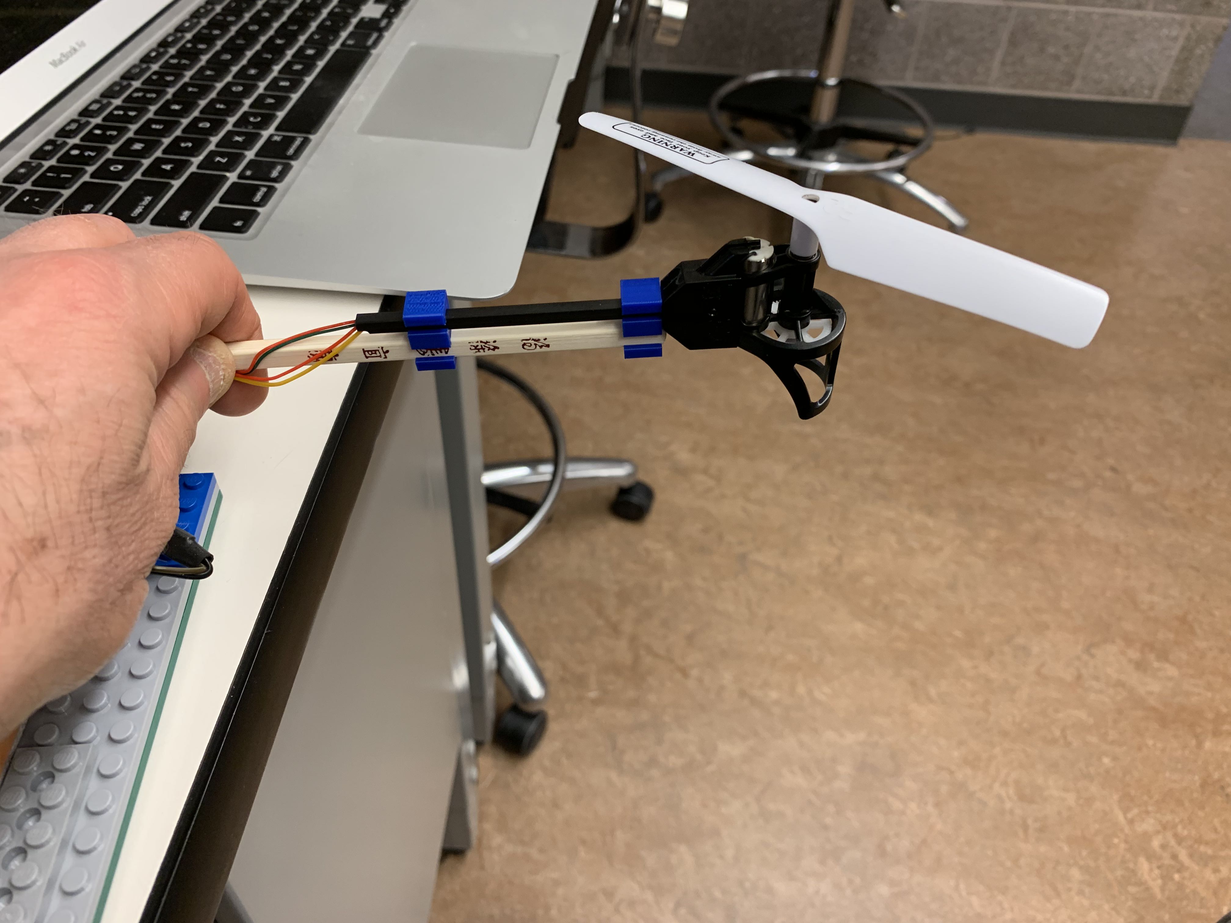
Note, the reason we have you hold the propeller is that the static and dynamic relationship between motor command and thrust production is strongly affected by direction (whether the copter is blowing up or down), by surroundings (like whether the airflow is blocked by a table or not), and by whether the is moving simultaneously. Hold the propeller in a nearly horizontal position (and with no airflow blockage, so off the edge of the lab bench) is the best way to get a good plot of the spin up waveform.
Once you have determined the model relating motor command to rotational acceleration, you can switch back to the PID control sketch.
Lets first see the impact of including the extra pole with a prescribed example. What is the period of oscillation of the step response in units of samples with our original model (no extra pole) when dt=0.001,kp = 20, kd=0.5,ki=0, mBack=3, and \gamma = 15. You can use the matlab script we provided to answer this question to answer this question.
It will be hard to go much further until we have fit your system by adjusting \gamma and 'tweaking' p. That's next!
Experiment: Estimate Your System
In the PID control sketch, at the top, set mBack to 3, m=3 in the difference equation model, and cmdNominal to the value that gives you an almost horizontal arm, set the togglePeriod to 2.0, the doToggle to true, and flash the control Teensy with the PID sketch.
With your system up and running, use the sliders to do the following:
- Use the sliders to set the Desired Angle to 0.05, the Integral Gain to Ki=0, and the Delta Gain to Kd=1.
- Use the slider to slowly increase the Proportional Gain, Kp, until your arm's step response clearly oscillates, and slowly settles. Note that when calculating the period of oscillation for the angle and error waveform plots on the browswer GUI, the sample period is one millisecond, the plot points are milliseconds apart (500 points is 500 ms). You can pause the GUI and zoom in on your browser to analyze your waveform.
- Use the slider to set the Proportional Gain, Kp=10, and find the smallest Derivative Gain, Kd, so that the arm oscillates but still settles down. Note the period of oscillation.
- Use the oscillation periods and rates of oscillation decay to estimate gamma and to slightly adjust the pole you just estimated.
Show a staff member how you determined the pole from the backEMF step changes. Then show a staff member your match between the physical system and the matlab model. How is the quality of fit with the added pole? How do your predictions compare to your experimental results? Are you able to predict the behavior of the propeller arm when you try values for Kp and Kd that are very different from the ones you used to fit the model (e.g. try Kp=20, Kd=3, does your model predict what your arm does) ? Explain the dominant factors for any differences?
THIS SECTION IS THE POSTLAB!!! YOU CAN GET A CHECKOFF IN OFFICE HOURS, OR AT THE BEGINNING OF NEXT WEEKS LAB!
In this section you will analyze our new closed loop system and conduct experiments to understand the model's predictive power.
For very small values of $K_i$, where is the new pole that the integral term introduced? How large must you make $K_i$ to have reasonably quick convergence of the steady state error to zero?
One possible approach is to start with K_d. Derivative gain is constrained by noise. How high could you reasonably set K_d without adverse noise performance? Then you can set a reasonable K_i by using a value that gave you good steady state convergence performance from your previous experiments. Given the other two, K_p can be optimized to improve the step response of the system. Once you determine a good K_p, try reoptimizing with K_i = 50, its maximum value.
- Use the sliders to set the Desired Angle to 0.1, set the gains to the values you designed.
- Run some of the experiments you did when you used an ad-hoc approach for picking gains. Have you improved your controller?
- How does the predicted behavior for your system (examine the calculated poles and plots of step responses) compare to the experimental behavior.
- Keeping K_p and K_d terms constant, what does your model predict as the highest stable K_i? What is the maximum K_i you determined from your model?
- How does a non-zero K_i affect the natural frequencies?
How did you pick K_d, K_p, and K_i? What are the best values of K_d and K_p if K_i = 50? How does the model match your experiments, explain any differences