Observers
Please Log In for full access to the web site.
Note that this link will take you to an external site (https://shimmer.mit.edu) to authenticate, and then you will be redirected back to this page.
This state-space lab our best attempt to focus on the most important aspects of the four state-space labs that make up a typical term in 6.302. We have adapted it to the fact that we do not have the opportunity to look over your shoulder and help you avoid pitfalls. As you will see, we have made significant use of simulation in matlab, and to reduce frustration, we have streamlined the process of moving controllers from matlab to the Teensy. The use of matlab here requires a local installed copy of matlab on your computer. Some of you have been using the online matlab, which you can continue to use (see the on-line matlab instructions below), but we encourage you you to install Matlab (following the instructions here).
In this lab you will return to the propeller-arm, but this time, you will use the simple PD controller to stabilize the arm, and then use its behavior to adjust the parameters of a discrete-time state-space (DTSS) model of the arm. Then you will use this calibrated DTSS model to explore pole-placement and LQR strategies for selecting gains for a measured-state feedback controller, and test candidate gain sets on your propeller-arm. As you will see, a key problem with measured-state feedback control is the noise in two of the state measurements, rotational velocity and backEMF. So you will switch to estimating states by using your calibrated DTSS model to simulate the propellor-arm system, and using the lower-noise angle measurements to correct the simulation. You will then explore explore strategies for selecting correction gains in your observer-based approach (the DTSS-based simulation of the system is referred to as an "observer"), with the goal of ensuring that the error in the observer's estimate of the states decays much faster than the tracking error in the state-feedback controller of the system. Finally, you will add a second propeller to your system, and demonstrate your observer-based controller on this much higher-performance system.
As you can see in the following video, observer-based control of the single propeller system is remarkably effective. Take particular note of the red and blue curves in the top three plots from the browser-based GUI on the computer screen, the red curves are the estimated states and the blue curves are the measured states. Note that the two track closely, but the estimated-state curves have far less noise.
The two propeller system with an observer-based controller can be quite impressive, such as in the following (somewhat cluttered) video, in which the two propeller system is rotating nearly 300 degrees. Notice again the close match between the measured and estimated states shown in the browser-based GUI running on the computer screen.
There are a number of key ideas in this lab, including:
- A good strategy for designing controllers is to use a simple controller to stabilize a system, so that you can take measurements and calibrate a state-space model, and then use the state-space model to design a more sophisticated controller.
- State-space models for physical systems are usually easiest to write down in continuous time, but conversion from continuous time (CT) to discrete time (DT) is a necessary step if one is designing an observer-based controller.
- In state-space, conversion from CT to DT is automatic and exact, assuming a piecewise constant control input (the zero-order hold). And since most microcontrollers generate piecewise constant outputs, the zero-order hold assumption is almost always satisfied.
- It is far easier to connect typical performance targets to relative state and input weights in a least-squares minimization procedure for determining feedback gains (LQR), than to connect performance targets to pole locations when using pole placement to determine feedback gains.
- Noise plays an essential role when choosing between measured-state and estimated-state feedback control strategies. Estimated-state strategies are particularly effective when one state measurement is far lower noise than the others.
- State estimates must converge quickly to avoid impacting controller performance, but increasing the correction gains for state estimation can magnify the impact of measurement noise.
The matlab scripts and the Teensy sketch to support this lab are all in one zip,
HERE.
IT IS ESSENTIAL that you keep all the files from the above zip in same directory, so that any updates you make to the matlab-based state-space model or to the controller can be transferred automatically to the Teensy. Automating the transfer makes it easier for you to "miss" some of the control design details, but eliminates the tedious and error-prone process of copying controllers by hand. Since this lab requires you to design many controllers, and we want you to explore alternatives, automation seemed to be the right tradeoff.
To use the automatic transfer, make sure that UseMatlabGenFile is set to true at the top of the Teensy 6302_SSMS_control sketch. Then run the matlab script propSS.m to simulate your model and controller, and plot the results. The script also generates a human-readable file containing a definition of your controller, obs6302.h. When you compile and download the sketch 6302_SS_control on to the Teensy, the compiler will read in the obs6302.h file, and download your controller on to the Teensy. DO NOT MANUALLY EDIT obs6302.h IN ARDUINO UNLESS YOU ARE USING THE ONLINE MATLAB AND FOLLOWING OPTIONS 2 SINCE IT WILL OVERWRITE THE CHANGES MADE BY propSS.m.
PRESS SHOW/HIDE TO VIEW THE INSTRUCTIONS FOR IF YOU ARE USING THE ONLINE MATLAB ONLY
- Download and install MATLAB Drive Connector, which can be downloaded from the MATLAB Drive page. Matlab drive connector allows you to keep a local synced copy of the files you edit in on-line matlab.
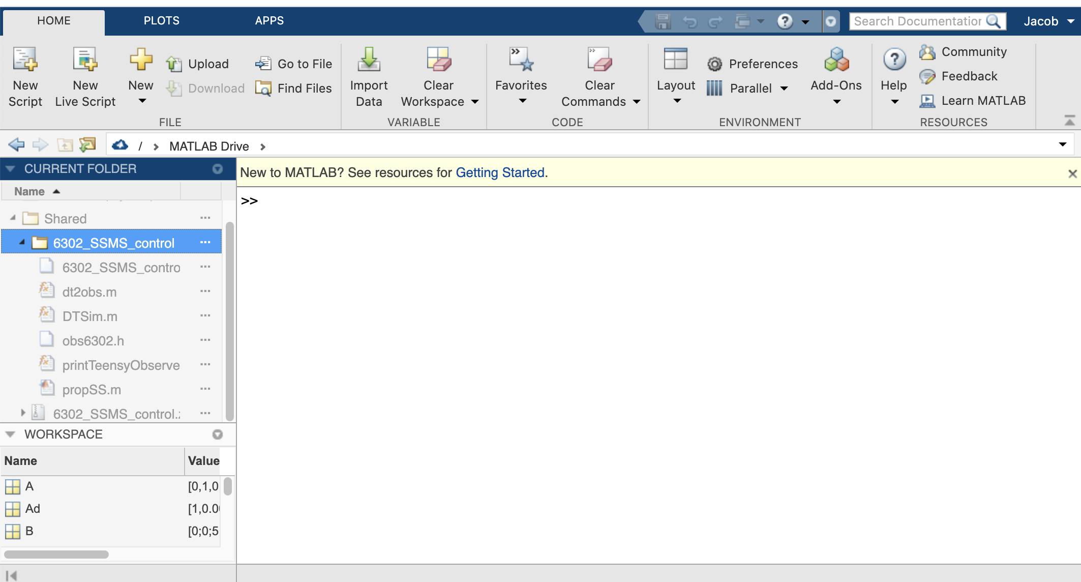
If you decide to use matlab drive connector, download and install it, and then start matlab connector. Then download the zip file for lab10, and copy it into the SHARED directory on your local matlab drive. Unzip the file, and then you should be able to see the matlab files in the on-line matlab, like in the screenshot below.
Use Teensyduino to open the 6302_SSMS_control sketch in the SHARED subdirectory of your local matlab drive. If the matlab connector is working properly, when you run propSS.m in the on-line matlab, the syncing should update your local version of obs6302.h. Then when you compile and download the 6302_SSMS_control sketch from the local matlab drive on to the Teensy 3.6, it should pick up the synced, updated, obs6302.h file.
- The other option is to have two copies of obs6302.h , one uploaded to online matlab (along with all the files in the zip downloaded above) and another copy on your computer in the same directory as the 6302_SSMS_control.ino file. Then, EACH time you run propSS.m the copy of obs6302.h uploaded to online matlab will get updated and then you will copy over the contents of to the local copy of obs6302.h on your computer.
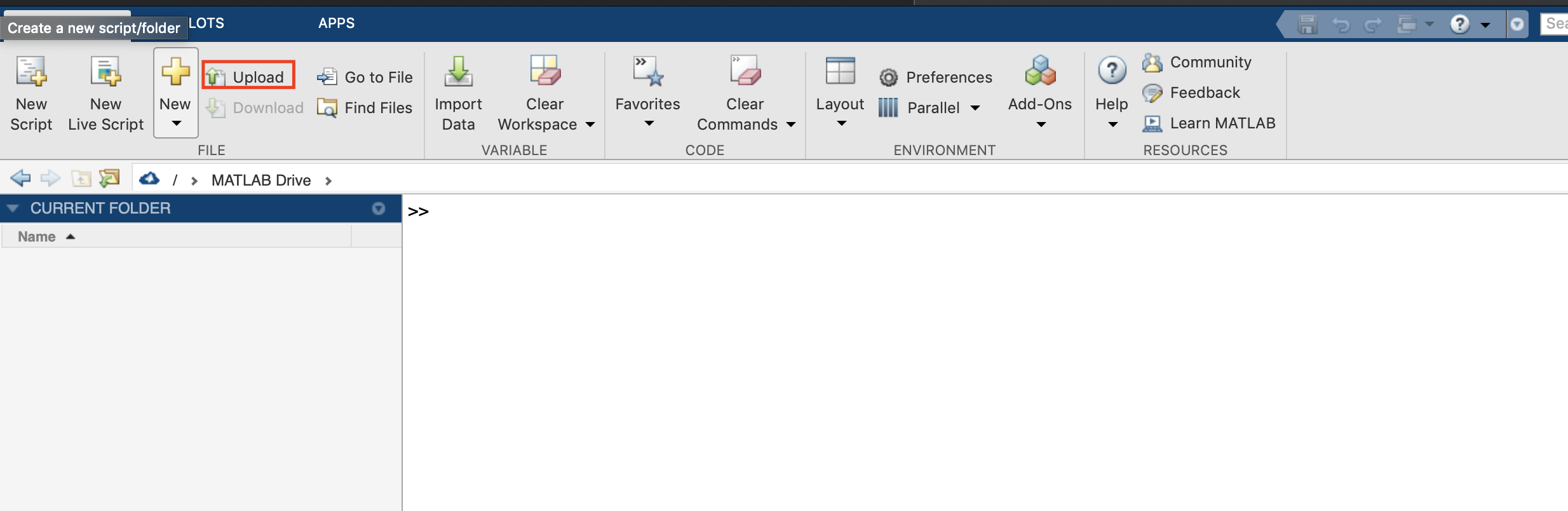
Step 1: Upload the contents of the zip file to online matlab
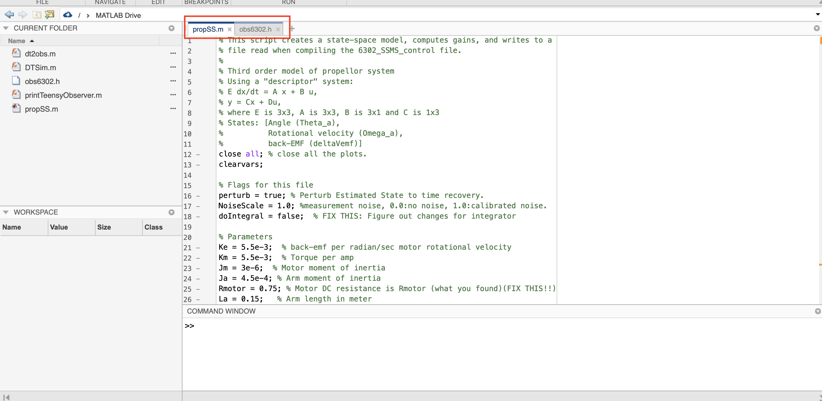
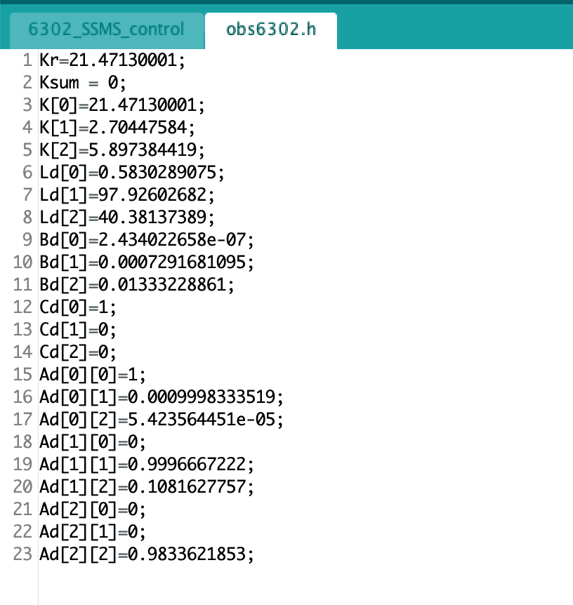
Step 2: Open the $propSS.m$ and $obs6302.h$. Run $propSS.m$ to generate updated parameters in $obs6302.h$
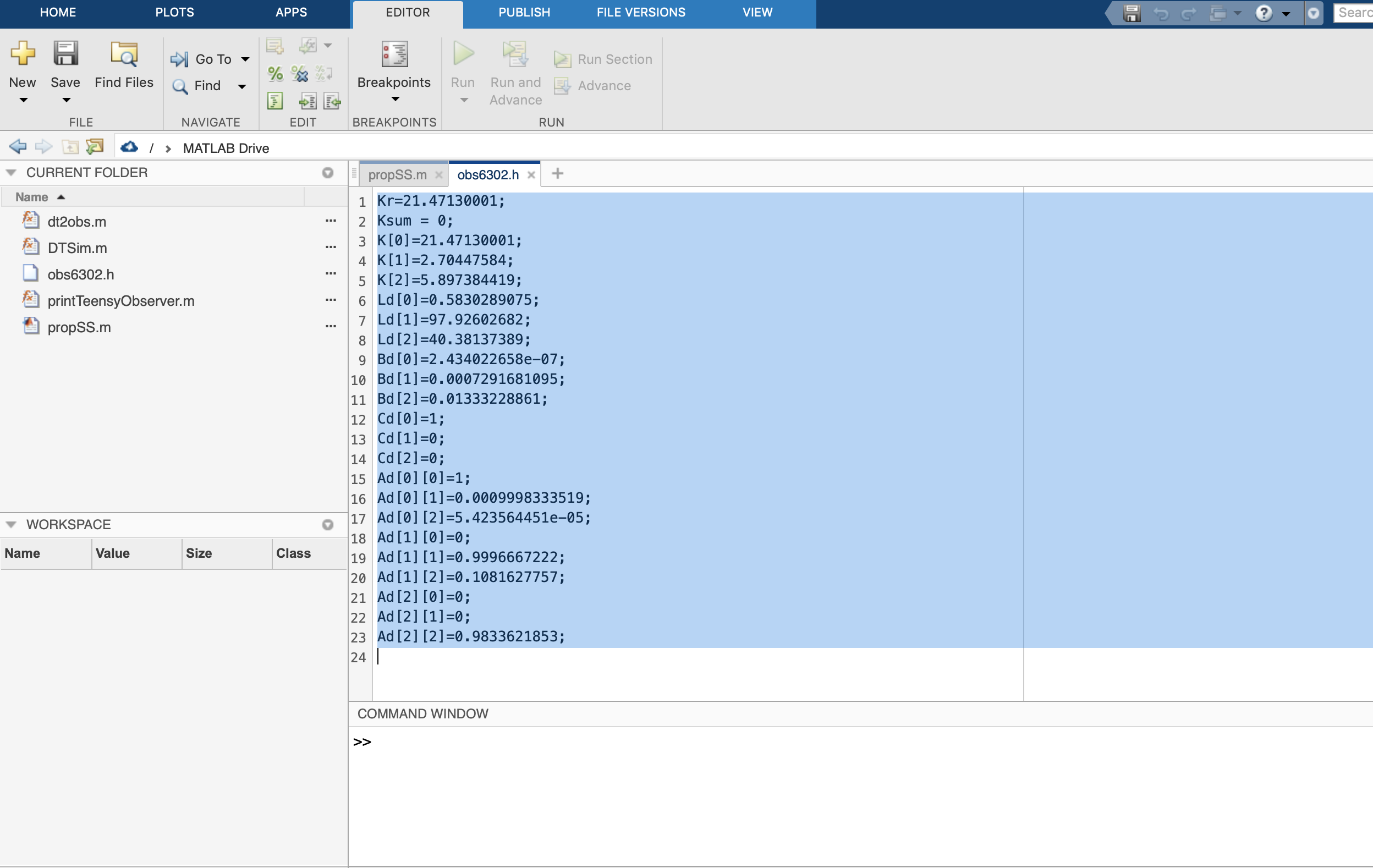
Step 3: Copy the contents of $obs6302.h$
Step 4: Make sure 6302_SSMS_control.ino and $obs6302.h$ are downloaded on your computer. Notice this copy of $obs6302.h$ is NOT the $obs6302.h$ that is you uploaded to online matlab, but you want to copy the contents from the updated $obs6302.h$ on the online matlab to the $obs6302.h$ that is on your computer.
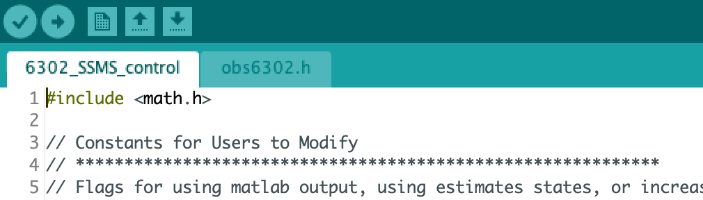
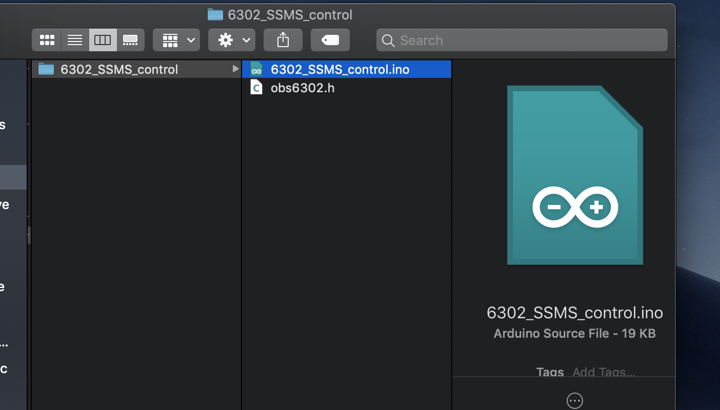
Step 5: When you open 6302_SSMS_control.ino you should see a tab for both 6302_SSMS_control.ino and $obs6302.h$
Step 6: Click on the $obs6302.h$ tab and paste the contents that you copied from the online version of matlab to the file in arduino. Save and upload and your teensy should have the latest gains generated by $propSS.m$ now.
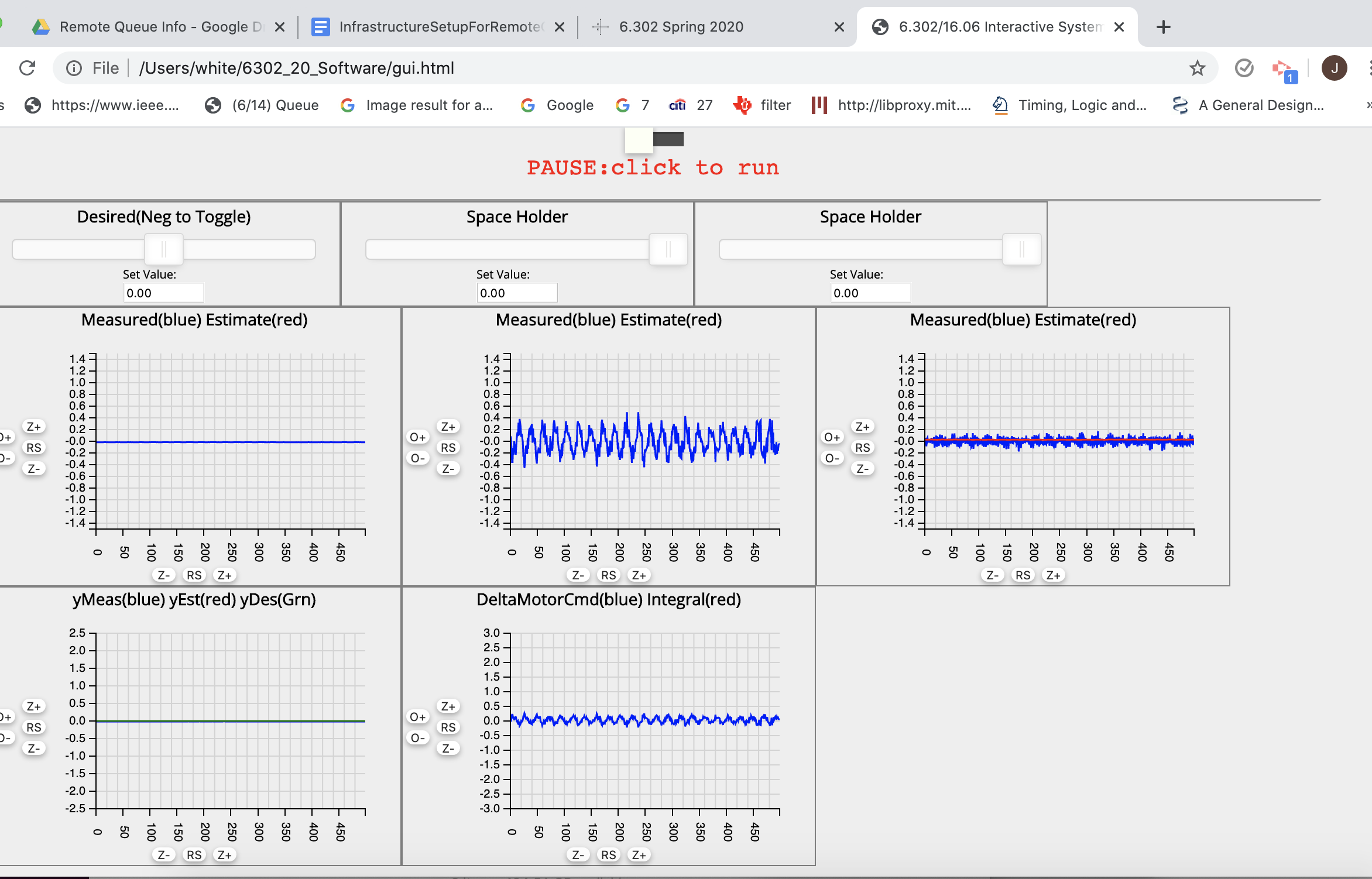
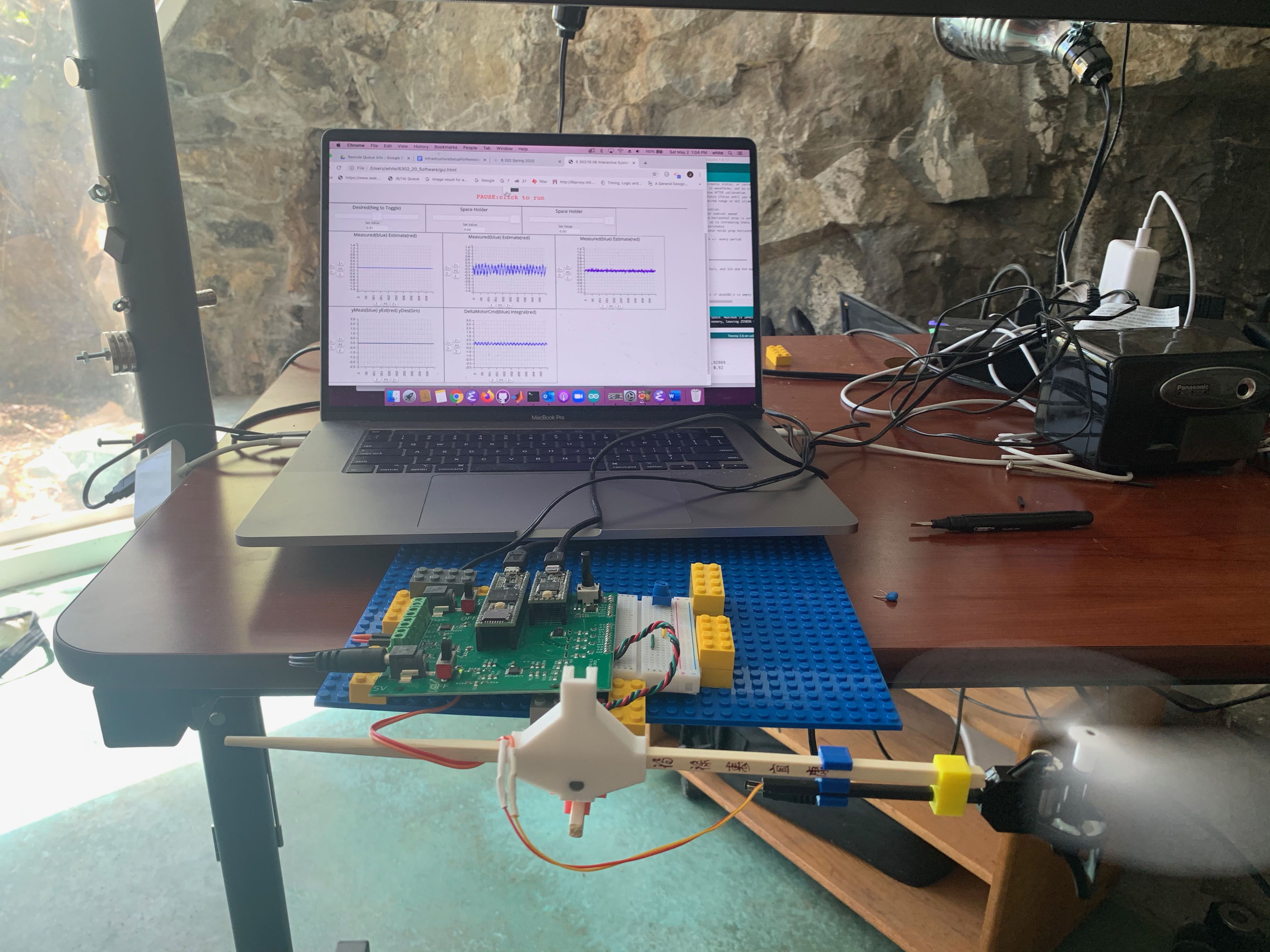
After running the propSS.m script in matlab and downloading the 6302_SS_control sketch on to the Teensy 3.6, start the python server, and open up the browser GUI. You should see three sliders and five plot windows, as in the picture below. The top row of three plot windows are plots of the three propeller-arm states (theta, omega and backEMF). Each window shows two plots, one for the measured state and one for the estimated state, though the estimated states will be zero until you set up the observer in check-off three below. The bottom row has two plot windows. In the left window, there are three plots, the measured output y in blue (theta in our case), the estimated output in red, and the desired output in green (the desired output is set by the leftmost slider). In the right window of the bottom row, the motor command and the integrater state are plotted (it is the delta motor command, so it is zero when the motor command is equal to its nominal value).
Note that is a total of 11 plots, and it should look like the picture below.
The are four major design tasks in this lab, associated with four checkoffs. Each checkoff is summarized below, and more details for each checkoff are in the sections that follow.
This first checkoff is intended to ensure you have a working, calibrated arm and associated state-space model before you start designing controllers. For it you will:
- Build the arm (there are detailed video instructions) below.
- Download the software for this week, run the matlab file propSS.m in the 6302_SSMS_control directory, upload the 6302_SSMS_control sketch to the Teensy 3.6, start the python server, and open up the browser GUI.
- Calibrate your arm's angle sensor offset, nominal command, Rmotor and backEMF offset.
- BE SURE to transfer the value you found for Rmotor when calibrating the propeller's backEMF to the matlab file propSS.m. Then rerun propSS.m to update the simulation.
- If your calibration is reasonable, then the GUI's 11 plots in five windows should look like the picture below. We know, 11 plots is a lot, but we need 6 plots to show measured and estimated theta, omega and BackEMF, 3 plots to show the measured, estimated and desired output y, a plot for the motor command (so you can see if it saturates) and an integrator plot (in case some want to play with it).
Below is a calibrated setup:
You will compare using pole placement and LQR-weight-selection when optimizing the step response under measured-state feedback control.
- Be sure that the flag UseMatlabGenFile is set to true and that the UseEst flag is set to false (and the biggerStep flag is also false) at the top of the 6302_SSMS_control sketch.
- You should find all the lines in dt2obs.m that say FIX THIS before line 30 (the observer starts on line 30, you will fix that part for checkoff 3), and fix them.
- Determine feedback gains using pole placement (these will be discrete-time poles) and setting LQR weights (in discrete-time, the matlab function is dlqr). In general, LQR determines gains by minimizing a weighted sum of squares, where the sum is over the states and the input. If you put a large weight on the input (by changing R), what will that do to motor commands? If you put a large weight on rotational velocity (omega), will the arm move quickly? Can you make the same connections between performance and pole locations?
- Run the propSS.m script to simulate your model and controller, and see if your changes had the intended effect. You should only look at the plots of the measured-state feedback, you will look at the estimate-state feedback plots in checkoff 3. Remember that the script also generates a human-readable file containing a definiton of your controller, obs6302.h.
- When testing a controller on the propeller arm, compile and download the sketch 6302_SS_control on to the Teensy. Be sure you run propSS.m in matlab first, so that the Teensy compiler will read in the latest obs6302.h include file, and download your controller on to the Teensy.
- Try setting NoiseScale to 1.0 (on line 17 in propSS.m), and rerun the script. What happens to the plots for the measured-state feedback system (you have not set up the estimated-state feedback system yet, so ignore those). What is to point of the vector of three values on line 76 in propSS.m? And lines 59 and 68 in DTSim.m?
- Be sure to try steps of various sizes, and watch the command window. What is the relationship between the R weight and the motor command. Can you set R to avoid saturating the motor command at all? If you pick an R so that the gains give you NO motor command saturation when you set the desired slider to -0.1, how is the performance? What if you allow the motor command to saturate during a transition, as long as it is not saturated once the arm settles to steady state?
Below is a video of one of our measured-state feedback controllers.
For this checkoff, you will determine gains for observer-based state estimation, and use them for your controller. The key issues will be ensuring fast convergence of the estimates, while keeping the noise low. You will be able to simulate the behavior, but the simulation does not include all the non-idealities of your propeller-arm system, so its predictions about how fast the state estimates converge will be informative, but probably optimistic.
- Be sure that flag UseMatlabGenFile is set to true AND that the UseEst flag is set to true (and the biggerStep flag should still be false) at the top of the 6302_SSMS_control sketch.
- You should find all the lines in dt2obs.m between 30 and 50 that say FIX THIS (the integral starts on line 50, adding the integral is interesting, but definitely optional), and fix them.
- You will have to decide how to pick the gains for converging the observer estimates, the Ld's. You will probably use either matlab's place or dlqr command, but you should think carefully about what those commands take as input, and what they produce as output. The estimator gains should depend on Cd, not Bd, but Cd is the wrong shape (Cd is 1xn, but Bd is nx1). Also, place and dlqr return feedback feedback gains, which are the wrong shape (K is 1xn, Ld is nx1). The matlab tick (') command transposes matrices, so Cd' is the transpose of Cd, but Cd is not the only matrix or output you will need to transpose.
- Run the propSS.m script to simulate your model and controller, and see if your changes had the intended effect. Try setting the perturb flag to true at line 16 at the top of the propSS.m file, and rerun the simulation. Do you see the change? The perturb flag causes the simulator to zero out the estimated state about 3/4's of the way through the simulation, to make it easier to see how fast the estimation error decays.
- Try setting NoiseScale to 1.0 (on line 17 in propSS.m), and rerunning propSS.m. How does the resulting noise depend on the estimator gains? What if you try to force the state estimates to converge very fast, what happens to the noise?
- Once again, the script generates the file obs6302.h which contains the definiton of your controller, including the observer model and the estimator gains. So when you compile and download the sketch 6302_SS_control on to the Teensy, the compiler will read in the latest obs6302.h include file, and download your controller on to the Teensy, including the observer model and the estimator gains.
- Pick "good" Kd's and Ld's, run propSS.m, then download 6302_SS_control on to the Teensy, run the python server and open up the GUI. Set the slider to toggle a small step (-0.05, for example), and compare the estimated states to the measured states in the top three plots (the red and blue curves). Do they match well? Try other step sizes.
- What happens when you set the desired slider to 0.2 (a bigger step)? If the motor command saturates, are your state estimates accurate? Look at lines 611 through 622 in the Teensy sketch, where the state estimates are computed. Can you move a few lines of code so that the estimator is more accurate when the motor command saturates?
- You can quickly compare estimated-state feedback to measured-state feedback by toggling the useEst flag at the top of the Teensy sketch from true (use the estimated states) to false (use measured states). What changes when you switch back and forth? Which is better and why?
Below is a video of one of our estimated-state feedback controllers.
For this checkoff, you will add the second propeller (video instructions below), modify the Teensy sketch to drive the second propeller, update the matlab state-space model, recalculate feedback and estimator gains, and then download the model and gains on to the Teensy. We suggest you review the end of prelab09, https://eecs6302.mit.edu/spring20/prelabs/prelab09/model.
- Make sure that the UseMatlabGenFile flag is true and the useEst flag is true.
- How do you update the arm friction you added for checkoff 1?
- Remember to FIRST run propSS.m to update the controller model and gains, and then download the 6302_SSMS_control sketch to the Teensy!!!
- Got a good controller? Are you Brave? Take off the training wheels (see below), set the biggerStep flag at the top of the Teensy sketch to true, reupload, and SLOWLY move the desired slider to the negative end of the range. BE PREPARED, if your controller's step response overshoots, your two propeller system could literally, literally, spin out of control.
We hope the following short videos will guide you quickly through setting up your propeller arm. As mentioned in the first video, it will be much easier to work together on zoom if you build the arm the same way we did, and in addition, the models we give you for your arm will likely be a better match. The model will not be perfect, but in the first checkoff you can improve it.
In a "very optional" lab11, you can run an algorithm that learns a model from measured frequency domain data generated by your arm, and then uses that learned model to do the control. It is very cool to see, for those who have time, or may want to try after you are finished with finals (I'll be available to help).
But first things first...
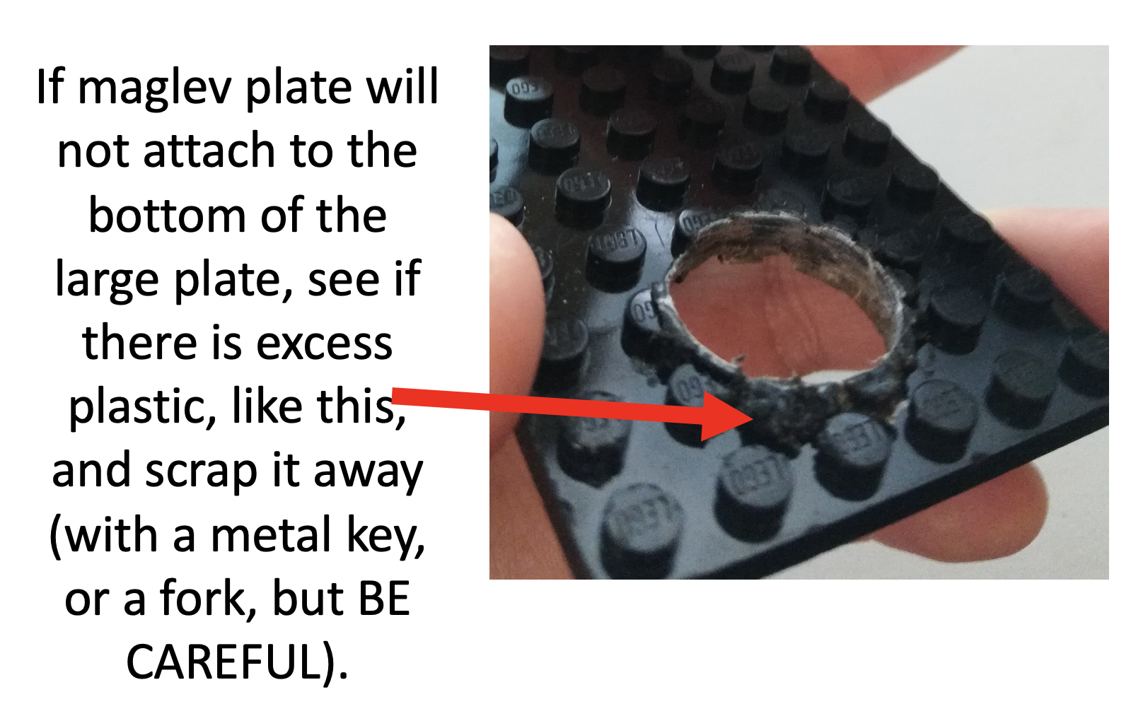
Before attaching the angle sensor in the next step, check the maglev plate for excess plastic (a result of drilling the hole in the plate for the bolt). If there is a lot of excess plastic, the plate might not attach easily to the bottom of the big base plate. See the picture below.
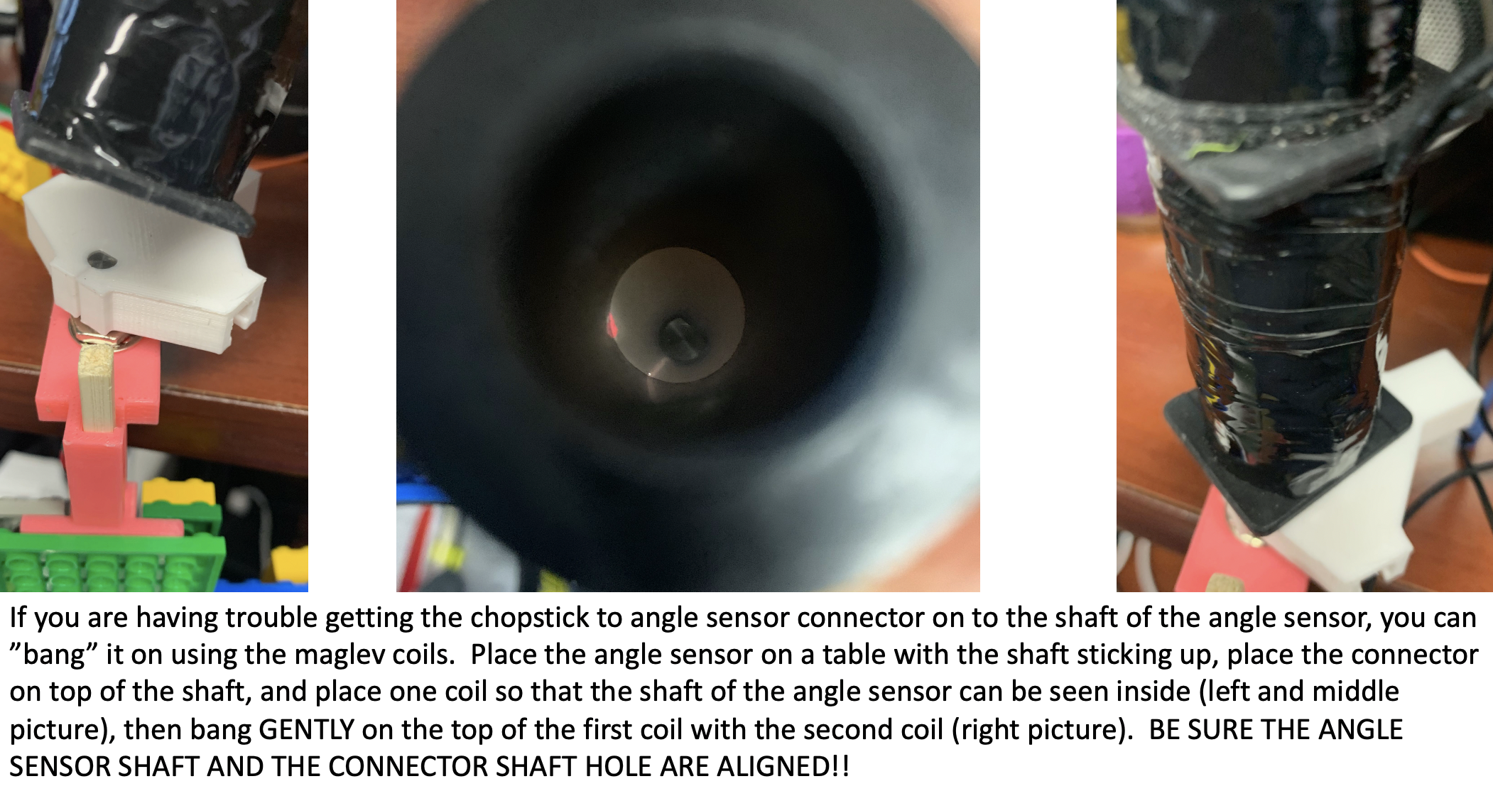
If you have trouble attaching the connector that holds the chopstick and attaches to the shaft of the angle sensor, you can use the two maglev coils to "bang it on," like in the picture sequence below.
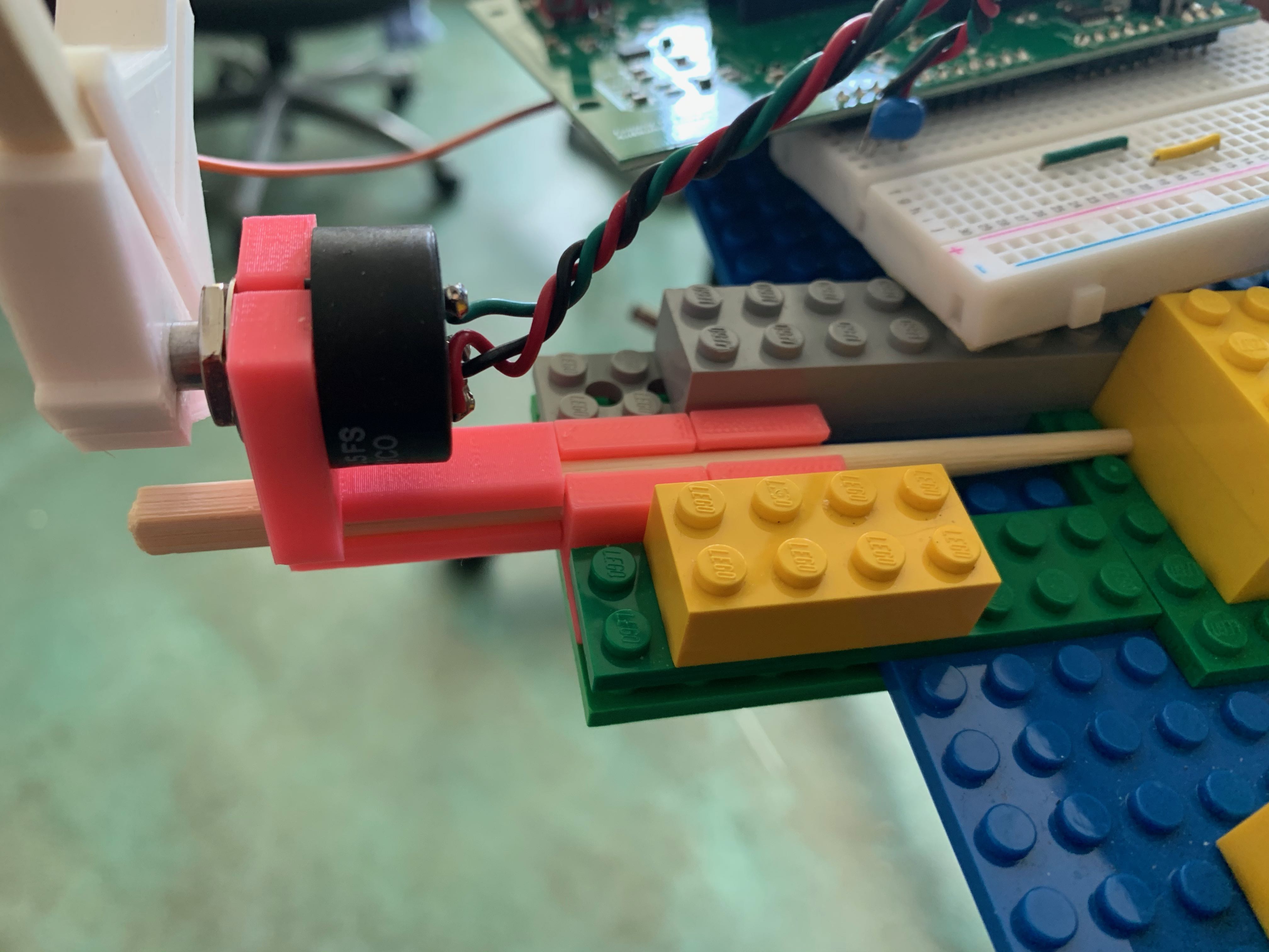
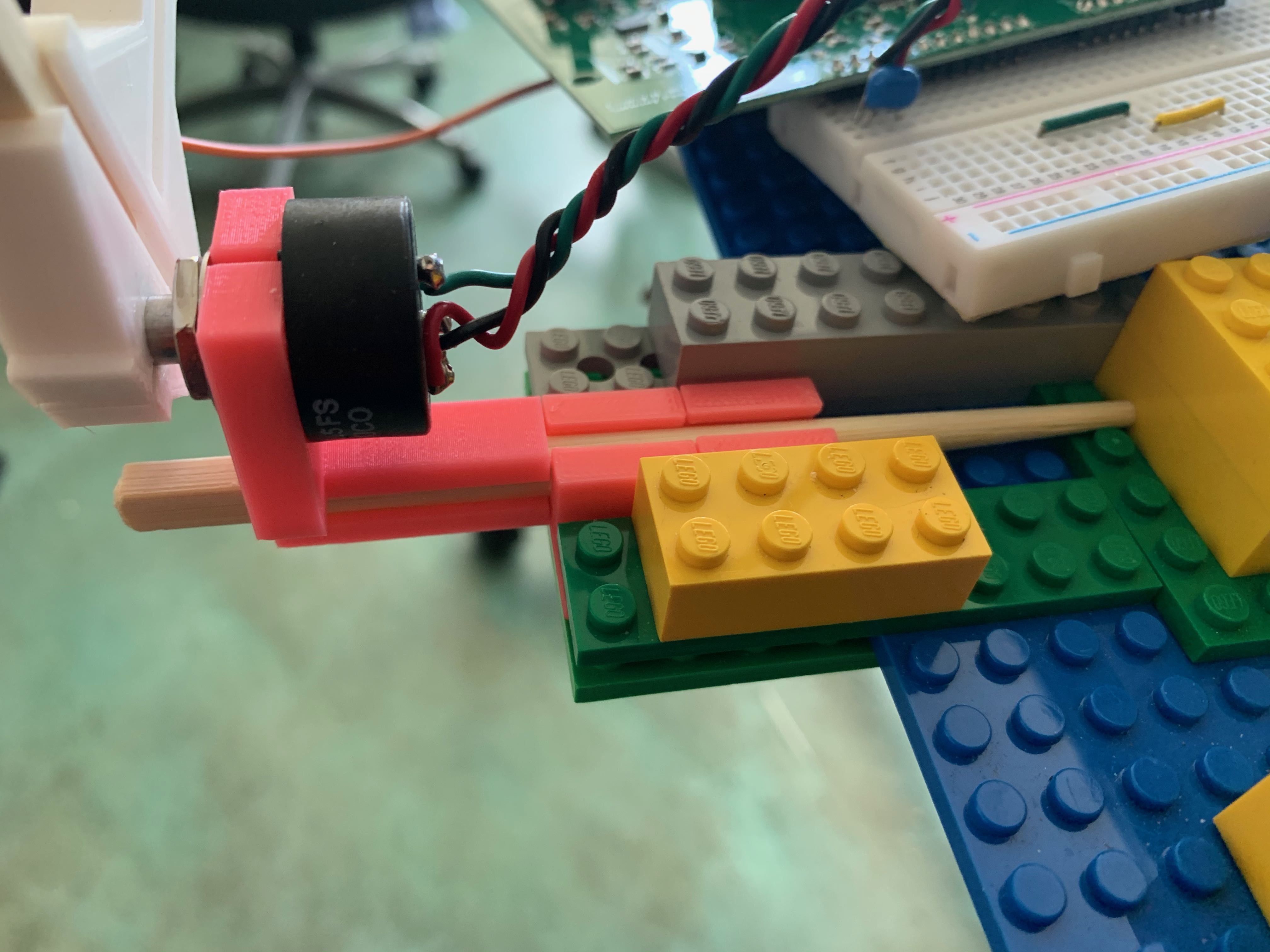
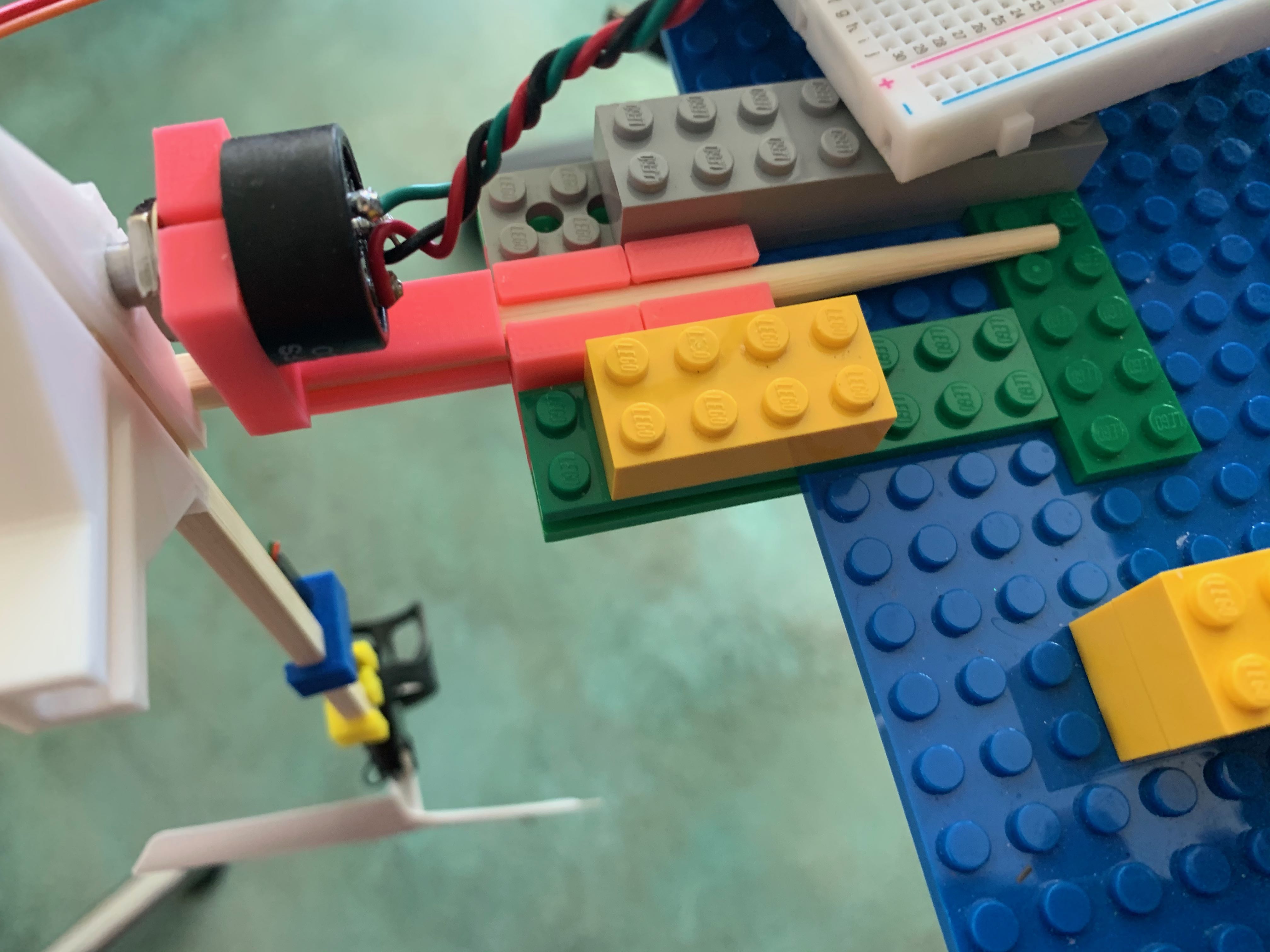
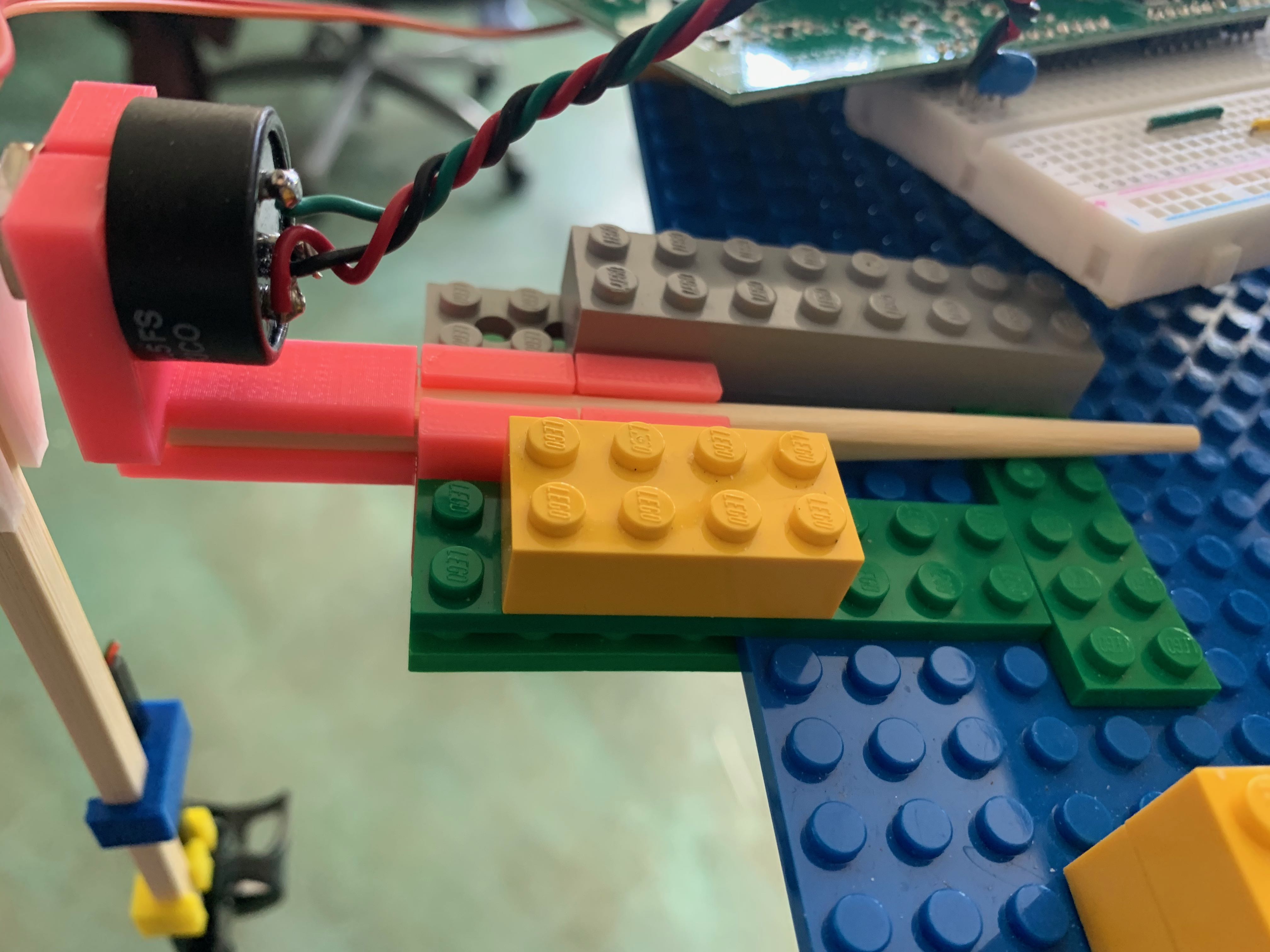
If you have trouble pushing the angle sensor on to the short chopstick, it can help to push up against a lego brick, like in the picture below.
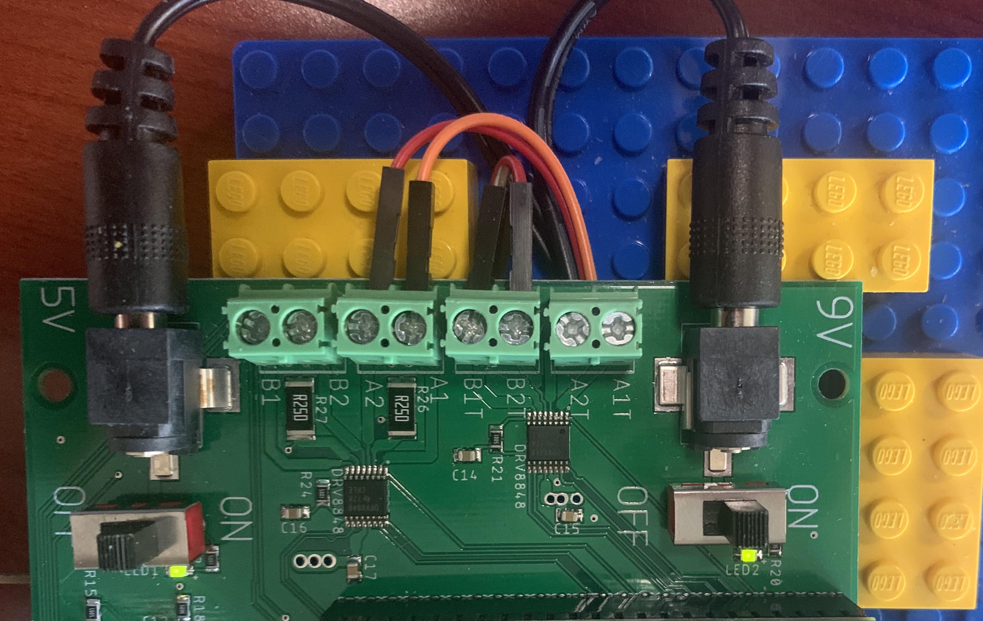
NOTE!!!!! There is a correction to this video, the propeller is connected to A1 and A2, not B1 and B2, see the picture below.
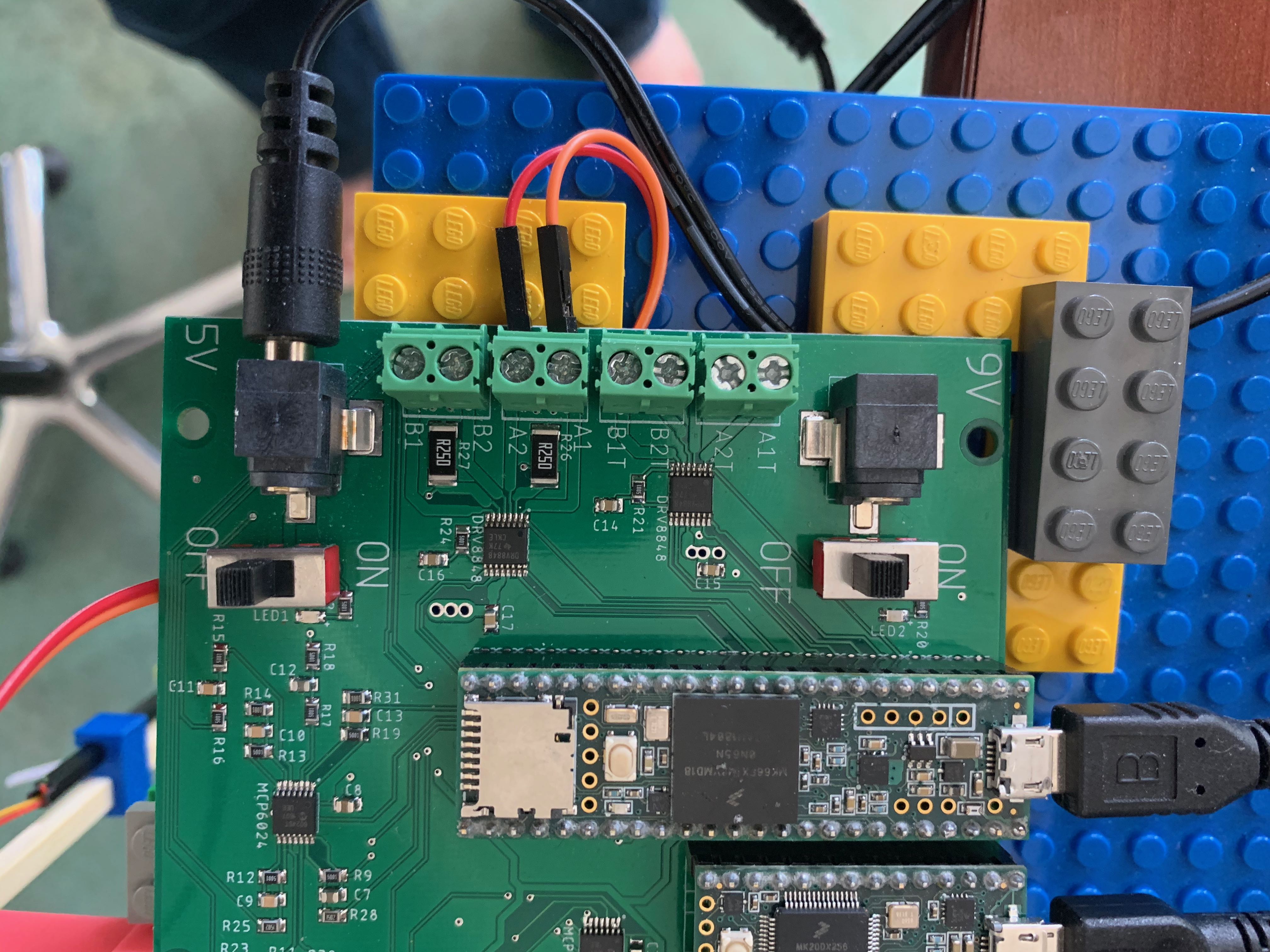
NOTE!!!!! There is a correction to this video, the propeller is connected to A1 and A2, not B1 and B2, see the picture below.
In the Teensy sketch at the top of this lab, the parameters for a low-performance PD controller (KpInitial 2.0 and KdInitial 0.5) are ALREADY SET. Use these values to hold the arm horizontal whenever you calibrate. Note that you should recalibrate every time you start working with the arm, as the propeller does change over time, and calibrating with a low gain PD controller is quick and reliable.
Remember that every time you change a value in the Teensy code, you must reflash the control Teensy. YOU SHOULD NEVER HAVE TO CLOSE THE BROWSER WINDOW, OR DISCONNECT, OR REFLASH THE MONITOR TEENSY. You should NOT need to restart the monitor every time you reflash the Teensy, but if you do, then something is not working properly and your time is being wasted, so you should ask for help.
First lets recalibrate the angle sensor and set the cmdNominal term to hold the arm horizontal.
- Step 0: Flash the Teensy, start the python server, start the browser GUI, and orient the set up with the arm hanging off the table, as in the picture of the setup above.
- Step 1: Set the thetaSensorOffset so that the angle plot in the browser (second row, leftmost plot window, blue plot) reads exactly zero when you hold the propeller arm (with your hand if necessary) exactly horizontal. Insure that the thetaSign is set to 1 or -1, whichever gives you a positive angle when you move the arm above horizontal.
- Step 2: Adjust cmdNominal in the Teensy sketch to the voltage needed hold the arm perfectly horizontal (zero angle). A reasonable cmdNominal is between 2.0 and 4.0, if you need a higher value, then something may be wrong with your propeller. MAKE SURE THE PROPELLOR IS BLOWING AIR DOWNWARDS, and if it is, then examine the white or red plastic propeller blade for damage, or better yet, ask help. NOTE: if everything is working correctly, the controller will keep the arm from flying away, so you should not be holding the arm.
- Step 3: Stop the propeller with your finger (thumb on the rotor will do nicely), and see if the backEMF plotted in the browser is almost exactly zero (within 0.05 volts). If positive, increase Rmotor, if negative, reduce Rmotor. Typical values for Rmotor are between 0.5 and 2.5, if you are finding values outside this range, ask for help.
- Step 4: If you correctly determined thetaSensorOffset, cmdNominal, Rmotor and the arm should be holding itself perfectly horizontal, then the blue plot in the second row, leftmost window, should read zero. Check that this is the case, and then complete the thrust linearization calibration below.
As described in the prelab, we can construct an approximate linear state-space representation of the propeller-arm system by linearizing any nonlinear relationships about the states when the arm is horizontal. And in particular, we had to linearize the relationship between backEMF and thrust about the backEMF voltage associated with the gravity-balancing thrust. Since this linearization is being used in a matlab model to predict gains, the model must be reflected in the Teensy implementation, or we have little reason to expect that the model will give reasonable predictions of best gains.
If the propeller-arm is holding itself horizontal, then the propeller must be spinning at exactly the right speed to produce a gravity-balancing thrust. The most straight-forward approach to including the backEMF linearization in our Teensy implementation is to measure the backEMF voltage when the arm is holding itself horizontal, and then set the bemfNominal at the top of the Teensy code to that value. This bemfNominal is subtracted from the measured backEMF, near line 597, at the bottom of the Teensy code, to generate the third measured state of our linearized propeller system (the first two states are theta and omega, the arm angle and rotational velocity).
So, the last calibration adjustment you must make is to adjust bemfNominal on line 16 (which should have been ZERO when you were calibrating the other parameters) to the value of the blue plot in the rightmost window of the first row of plots in the GUI (that is a plot of the measured third state, the linearized backEMF). After you make the change and reflash, the backEMF reading when the arm is holding itself horizontal should be zero (within 0.05 volts). If not, readjust bemfNominal.
If you have calibrated your system then it is time to set appropriate gains to implement proportional+derivative control. But not so fast......
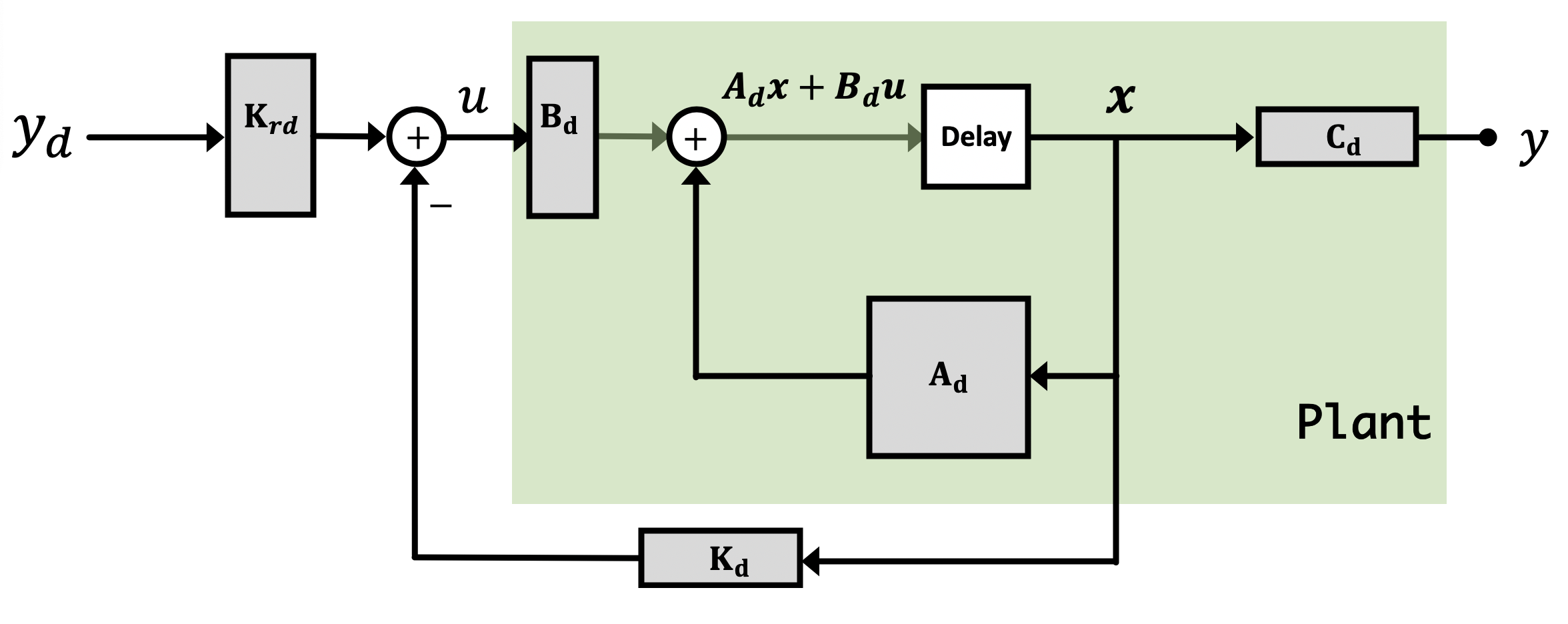
Implementing state feedback required a change to the way this Teensy code computes the motor command; the change has already been implemented and the relevant lines are between 603 and 609. The motor command is a weighted sum of states, with one weight, which we also call a gain, for each state of the three-state propeller model. There is also the input scaling, Kr, which scales the desired angle's contribution to the motor command so that, in steady-state, desired(\infty) - \theta(\infty) = 0. How will you change all these gains to implement PD control? If you are not sure how, please review the prelab or ask a staff member.
To test your understanding of the relationship between the PD controller and the state-space controller, and to test the automatic transfer from matlab to Teensy, set the UseMatlabGenFile flag at the top of the Teensy sketch to true, and set the PD controller gains by updating the Kd vector on line 23 of the dtObs.m matlab file, Krd at line 29 (the block diagram from the prelab is reproduced below to help you with this), and the Adcl in line 26. Run propSS.m, then upload 6302_SSMS_control on to the Teensy 3.6, and see if the gains you set in the matlab file change the step responses of the arm.
Once you have verified that changes in matlab are making their way to the Teensy, compare simulated and measured step responses for your propeller under low-gain PD control. Try a proportional gain of 2, and a derivative gain of 0.5, and then try reducing the derivative gain to 0.25 (in each case by changing the Kd vector in matlab, and then updating the controller on the Teensy by rerunning propSS.m, and reuploading the 6302_SSMS_control sketch). Try to improve the match between what you see in simulation, that is, the measured-State feedback plots, and the plots of the measured states (in blue) in the top row of plot windows in the GUI.
You will likely see that the measured behavior of the propeller arm is more stable than predicted by the simulation in the low PD gain setting, please try to improve the match by adding arm friction to the matlab state-space model in propSS.m. Where will you put the arm friction? Be sure to test your added arm friction for several different step sizes (by setting the desired slider on the GUI to different negative values), and carefully monitor the motor command plot (second row, right side, in blue). If the motor command "saturates", then your linear model will not match, regardless of added friction.
YOU MUST BE ABLE TO ANSWER ALL THE CHECKOFF QUESTIONS IN ORDER TO GET THE CHECKOFF!!!

In the matlab script, propSS.m, we implemented a state-space model for a nominal propeller arm. That script calls the function dtObs to design a controller, then calls the function DTSim to simulate the system and controller, and finally calls the function printTeensyObserver to generate the include file for the Teensy sketch. If you examine the function dtObs, defined in the matlab file dtObs.m, you will see that it is "unfinished" (try running propSS.m, which calls it). You fixed a few of the errors before checkoff 1. Now go through and find what we "forgot" to finish by searching for FIX THIS in the matlab code. Please fix the matlab script, and then use it to find gains for your system. Then you can try on the propeller and see how well they work.
Well, "fix the matlab script"? That was a little glib.
Months ago, when we first used PD control, we eyeballed gains or we created models to help us search for good gains. We would now like to use a "somewhat" more systematic way of picking the values of \textbf{Kd}.
With full-state feedback, usually we can move the poles of the open-loop system, the eigenvalues of \textbf{Ad}, anywhere we want (not always, but that is a more advanced topic). That is, given certain conditions (which are met in this case), we can adjust the state-feedback gains to place the poles of the closed-loop system, the eigenvalues of \textbf{Ad}_{cl} anywhere we want. That is, by picking \textbf{Kd}, we can move
For second order systems, one can solve "on paper" for gains that will position your eigenvalues. For larger systems, beyond third order, there is no closed form for the eigenvalues, and finding the gains for a given pole placement is best done computationally. We can rely on numerical approaches for determining \textbf{Kd} given \textbf{Ad} and \textbf{Bd}, such as Ackerman's method and its variants. Matlab's place command does exactly what we want, provided we do not try to place poles right on top of each other,
% Ad = your Ad matrix
% Bd = your Bd matrix
p = [0.1 0.2 0.3]; % poles must be unique
Kd = place(Ad,Bd,p)
Unfortunately, even though we have a function that will take desired eigenvalues(aka poles) and return the needed gains, that does not mean we can just set the closed-loop eigenvalues to be real and put them at 0. If we could, then our system would match any desired angle in one step, and who wouldn't want that? For example, what gains do you get if you try to set the closed-loop poles for our system to 0.1, 0.2, and 0.3?
If you examine the dtObs function, before line 30 (the observer design starts after line 30, and that is the next checkoff), you will see that we have set up most of what you need to try LQR. Since the system is in discrete-time, you use the matlab dlqr function, but you have to decide on state and input weights for the LQR-based gain selection (there is also code for computing the gains with the integral term, ignore that for now). In general, LQR determines gains by minimizing a weighted sum of squares, where the sum is over the states and the input. If you put a large weight on the input (by changing R), what will that do to motor commands? If you put a large weight on rotational velocity (omega), will the arm move quickly? It is not as easy to make similar connections between performance and pole locations.
While experimenting in simulation and on the propeller system, remember that this is an iterative process. You guess at weights, examine the simulation results, and then adjust the weights and examine again. Then try on the propeller, examine the results, and go back and readjust weights. When you are happy with the results, you should be getting performance similar to the video in the summary section for checkoff 2, repeated below:
Below is a video of one of our measured-state feedback controllers.
A few things to keep in mind:
- Be sure that the flag UseMatlabGenFile is set to true and that the UseEst flag is set to false (and the biggerStep flag is also false) at the top of the 6302_SSMS_control sketch.
- You should find all the lines in dt2obs.m that say FIX THIS before line 30 (the observer starts on line 30, you will fix that part for checkoff 3), and fix them.
- Try using pole placement and setting LQR weights to determine gains for your controller.
- Run the propSS.m script to simulate your model and controller, and see if your changes had the intended effect. You should only look at the plots of the measured-state feedback.
- Compile and download the sketch 6302_SS_control on to the Teensy. The compiler will read in the latest obs6302.h generated by running propSS.m, and download your controller to the Teensy.
- Try setting NoiseScale to 1.0 (on line 17 in propSS.m), and rerun propSS.m. What happens to the plots for the measured-state feedback system (you have not set up the estimated-state feedback system yet, so ignore those plots). What is the point of the vector of three values near line 76 in propSS.m? And lines 59 and 68 in DTSim.m?
- Be sure to try steps of various sizes, and watch the command window. What is the relationship between the R weight in dlqr and the motor command. Can you set R to avoid any saturation of the motor command? If you pick an R so that the feedback system NEVER causes the motor command to saturate when you set the desired slider to -0.1, how is the performance? What if you allow the motor command to saturate somewhat?
YOU MUST BE ABLE TO ANSWER ALL THE CHECKOFF QUESTIONS IN ORDER TO GET THE CHECKOFF!!!
For this checkoff, you will determine gains for observer-based state estimation, and use them for your controller. The key issues will be ensuring fast convergence of the state estimates, while keeping the noise low. You will be able to simulate the behavior in matlab before trying it on the arm, but the simulation does not include all the non-idealities of your propeller-arm system, and does not include the realistic disturbances (like wind gusts, or the propeller hitting the edge of the table, etc), so its simulation of state estimate accuracy will be informative, but probably optimistic.
First, you should find all the lines in dt2obs.m between 30 and 50 that say FIX THIS (the integral starts on line 50, adding the integral is interesting, but definitely optional), and fix them.
Fix them? Being a little glib again.
To fix the observer part of the dtObs function, you will have to decide how to pick observer gains, the Ld's. You want to ensure fast convergence of the state estimates, as those estimates will be used in the state-feedback controller.
You must decide whether to use matlab's place or dlqr functions to compute the Ld's, but their application is not that straight-forward. You should think carefully about the fact that the estimator gains depend on Cd, but Cd is the wrong shape for dlqr and place (Cd is 1x3, but Bd is 3x1). And both dlqr and place return K's, which are also the wrong shape (Kd is 1x3, Ld is 3x1). The matlab tick (') command transposes matrices, so Cd' is the transpose of Cd, but Cd is not the only matrix you will need to transpose. And you might find the following transpose identity useful,
Once you have a strategy for determining estimator gains, run the propSS.m script to simulate your model and controller, and see if your changes had the intended effect. Try setting the perturb flag to true at line 16 at the top of the propSS.m file, and rerun the simulation. Do you see a change? The perturb flag causes the simulator to zero out the estimated state about 3/4's of the way through the simulation, to make it easier to see how fast the estimation converges. Then try setting NoiseScale to 1.0 (on line 17 in propSS.m), and rerun propSS.m. How does the resulting noise depend on the estimator gains? What if you try to force the estimates to converge very fast, what happens to the noise?
When you are satisfied that you have good gains, be sure that flag UseMatlabGenFile is set to true AND that the UseEst flag is set to true (and the biggerStep flag should still be false) at the top of the 6302_SSMS_control sketch. Then run the propSS.m script, as it will generate a human-readable file containing a definiton of your controller, including the estimator gains and new state-space model. Then compile and download the 6302_SS_control sketch on to the Teensy.
Once your controller is downloaded, try setting the desired slider to 0.05 (a small step), and compare the estimated states to the measured states in the top three plots (the red and blue curves). Do they match well? What happens when you set the desired slider to 0.2 (a bigger step)? If the motor command saturates, are your state estimates accurate? Look at lines 611 through 622 in the Teensy sketch, where the state estimates are computed. Can you move a few lines of code so that the estimator is more accurate when the motor command saturates?
To quickly compare estimated-state feedback to measured-state feedback, toggle the useEst flag at the top of the Teensy sketch from true (use the estimated states) to false (use measured states). What changes when you switch back and forth? Which is better and why?
You should be getting performance similar to the video in the summary section for checkoff 3, repeated below:
YOU MUST BE ABLE TO ANSWER ALL THE CHECKOFF QUESTIONS IN ORDER TO GET THE CHECKOFF!!!
Several weeks ago, you examined how to generate a state-space model for the two propeller system, and now we are going to finally use it! We suggest you review the end of prelab09, https://eecs6302.mit.edu/spring20/prelabs/prelab09/model. You will need to: add the propeller, modify the Teensy sketch to drive it, modify the matlab state space model for the two propeller system, determine feedback and estimator gains, and download the controller on to the Teensy. No problem!
In the video below, we show how to add the second propeller. Note that the video shows the first propeller connected to the incorrect positions!! The first propeller should remain in the A1 and A2 terminals! See picture below video.
Note the correct connections for the two propellers and two power supplies.
Once you have added the second propeller, modify the Teensy code to drive the two propeller system (note that the second propeller is driven by the second Hbridge, so you will also need the second five power supply). In particular, how will you change line 626 in the Teensy sketch to drive the second propeller? Should cmdNominal remain unchanged, and why? Once you have decided how to update the Teensy sketch, you can test your two propeller system with the sample simple low gain PD controller we used in checkoff 1. When you do, please make sure that both propellers are blowing air DOWN!!
Are far as modifying the state-space model goes, it is true that for a complete description of the two propeller system, you need four states: angle, angular velocity, and one backEMF voltage for each motor. BUT, if you are going to use an observer, and the observer must estimate the state based ONLY on angle measurements, will an observer be able to estimate two different backEMFS? Suppose both propellers are spinning at the same speed, but you do not know at what speed, can you tell from an angle measurement? Suppose the propellers are spinning at different speeds, can you detect the DIFFERENCE in speeds from angle measurements? NOTE: The concept of "Observability" is more general than this example, and is studied in more advanced control classes.
So, think about a three-state model of the two propeller system (Hint: think about driving the propellers with equal magnitude, but opposite signed, u's). Is it the same as the single propeller model? What would happen to that arm friction you might have added in checkoff 1? And once you have determined how to model the two-propeller system, modify the matlab state-space model accordingly, and use the matlab script to design controller and observer gains. Will you have to modify the LQR weights or pole positions you used for the single propeller model?
Once you have a good controller, make sure that the UseMatlabGenFile flag is true and the useEst flag is true, run propSS.m to update the controller model and gains, and then download the 6302_SSMS_control sketch to the Teensy.
So, have you got a good controller? Brave? Take off the training wheels (see below), set the biggerStep flag at the top of the Teensy sketch to true, reupload, and SLOWLY move the desired slider to the negative end of the range. BE PREPARED, if your controller's step response overshoots, your two propeller system could literally, literally, spin out of control.
Safety's On.
Safety's off!!!
Can you do as well as we did?
Show us your changes, show off your performance, make a video, and send it in to one of the staff!