1st-Order Differential Equations and Proportional Control
Please Log In for full access to the web site.
Note that this link will take you to an external site (https://shimmer.mit.edu) to authenticate, and then you will be redirected back to this page.
When we studied difference equations, we started with the first-order homogenous difference equation,
Solutions to first-order homogenous differential equations are quite similar. If
If
As we saw for DT systems, and we saw in prelab03 for CT systems, higher order difference or differential equation systems have natural frequencies that are roots of polynomials, so even real equations can have complex natural frequencies. But we will return to the higher-order case later, for now, let us consider an example of proportional feedback leading to homogenous difference or differential equations.
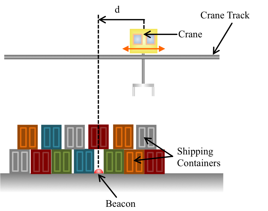
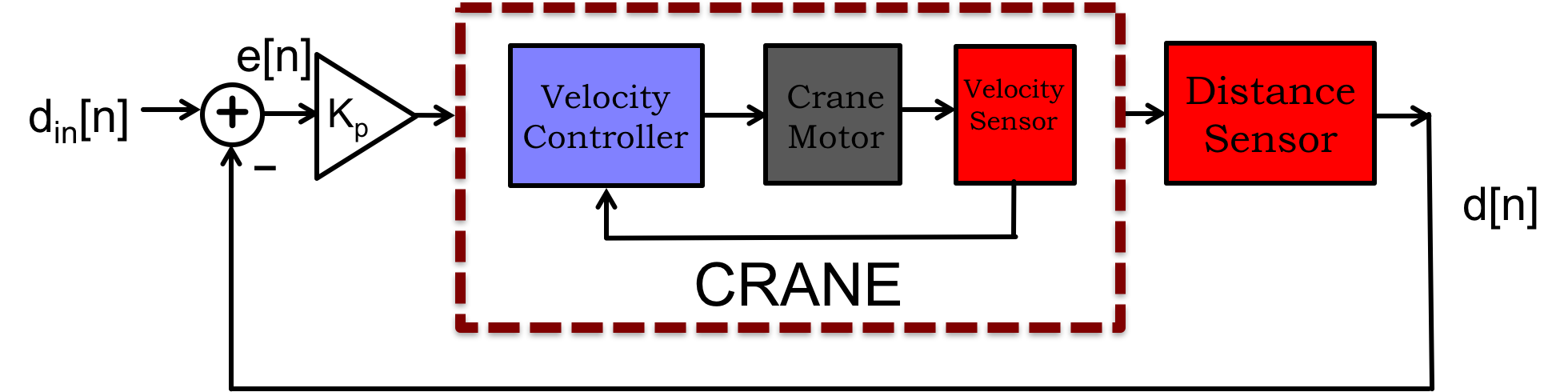
Let us return to the cargo crane traveling on track above a buried beacon, as shown in Figure 2. Suppose we must decide between two control systems, a discrete-time controller that measures distance to the beacon every \Delta T seconds, and a continuous-time controller that measures the distance continuously. One way to compare the two systems is to examine the problem of returning the crane as rapidly as possible to "home" position, that is, back to the beacon at d = 0. And for this comparison, we are going to assume that the crane has an internal feedback controller, one allows us to design a controller that senses position and controls crane velocity (as show in Figure 3 below).
For our velocity-controlled crane with discrete-time sensor,
If we use proportional control to return the robot back to the beacon (d=0), then the DT controller velocity at n \Delta T is given by
For the continous-time controller, crane distance and velocity are related by a derivative,
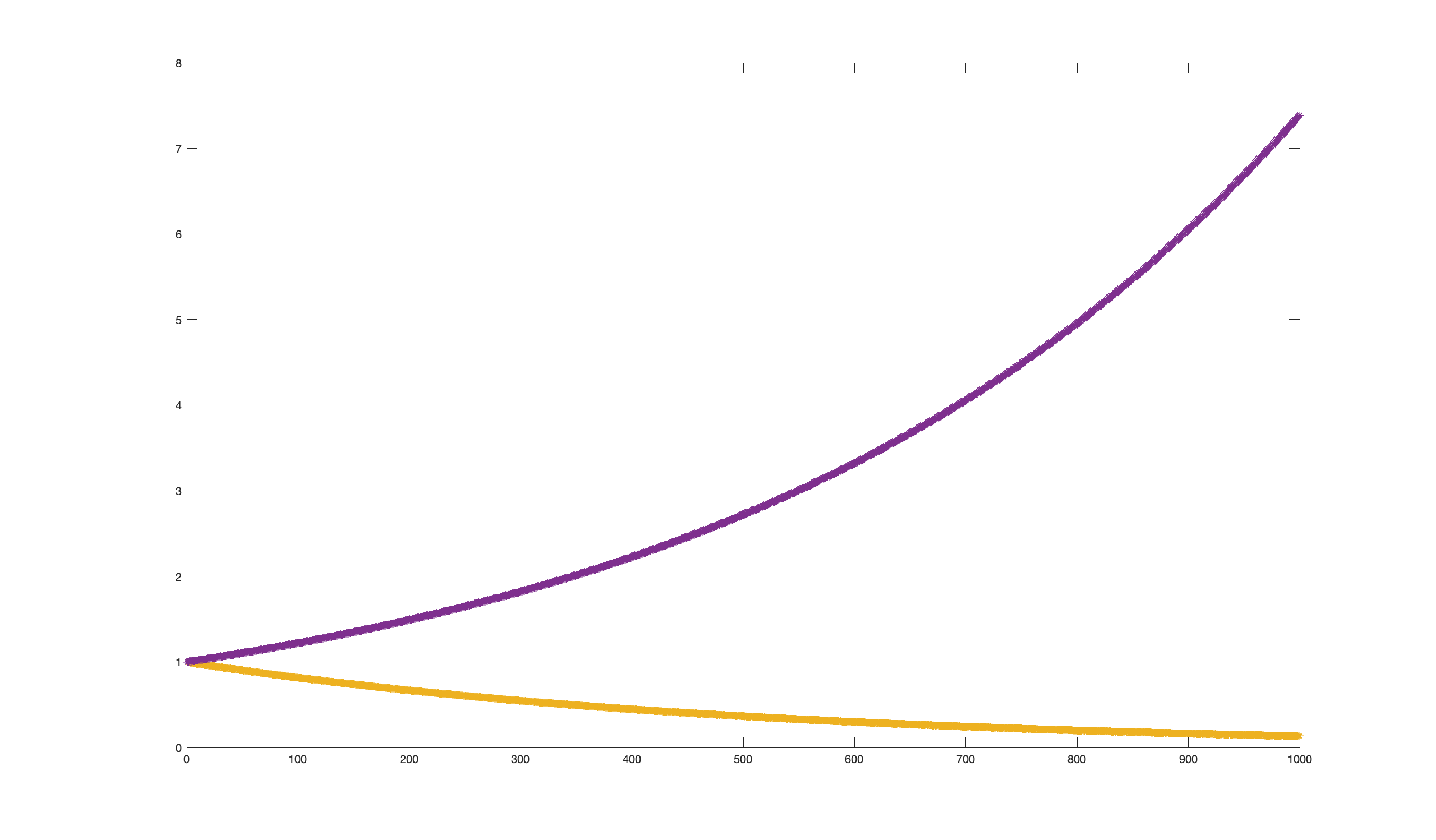
Suppose the cranes are being independently monitored with remote LIDAR, which measures the distance between the crane and the beacon every ten seconds. A test was run using the CT controller with an unknown proportional gain K_p, in which two consecutive measurements from the LIDAR system (which we can denote as d(t) and d(t+10)) gave distances of 200 meters and then 10 meters between the beacon and the crane.
What was the third consecutive LIDAR measurement, d(t+20), and to within one percent, what was the controller gain, K_p, in meters per second?

Suppose we want to test the DT controller with \Delta T = 0.1, then \Delta T = 0.5, and finally with \Delta T = 10 seconds. Determine the three values of K_p we should use if we want to match the measured performance to the CT system. That is, if d[n_0] = 200 meters, and n = \frac{10}{\Delta T}, then then d[n+n_0] = 10 meters (so n=100 for \Delta T = 0.1, n=20 for \Delta T = 0.5, and n=1 if \Delta T = 10). Determine the three gains, K_p, in meters per second (answers should be within one percent).
Suppose we know the same proportional gain, $K_p$, was used for a CT and a DT controller, and we know LIDAR monitor read $d(t) = 100$ and $d(t+10) = 10$ for the CT controller. What is the largest $\Delta T $ (of $\Delta T$'s that are an integral divisor of $10$) so that $d[n_0] = 100$, $d[n_0 + \frac{10}{\Delta T}] = 10 $ to within ten percent? This problem requires a bit of trial and error.
If \Delta T is small, so the sample rate for the DT system is fast, how close are the behavoirs of the DT and CT crane control systems? As we noted more generally above,
For example, in the CT crane control problem, we can pick a gain, K_p, that will reduce the distance to the beacon by a factor of ten in one millisecond. What would that gain be?
For the CT case, fast response corresponds to a very negative natural frequency, and in the DT case, fast response corresponds to a natural frequency whose magnitude is near zero. We can pick a K_p for the DT case that will give us a natural frequency of exactly zero, and ensure a one-step return to the beacon. Such controllers are sometimes referred to as dead-band controllers. What is the value of the natural-frequency-zeroing K_p as a function of \Delta T? (use a python expression, and use 'dt' to for \Delta T.)
How do the above $K_p$'s compare if the DT case has a one millisecond sample period? How do the distances from the beacon compare?
If \Delta T is small, then using the K_p which gives a DT natural frequency of zero can become impractically large. So it might seem like using a long \Delta T, like the \Delta T = 10 case above, would yield a zero natural frequency and a reasonable gain. But consider the crane velocity right before the update when moving from d[n_0] = 200 to d[n_0+1] = 5 meters. With K_p = 0.1, the velocity jumps from 20 meters per second to 0.5 meters per second, hardly smooth deceleration.
But there is a more serious issue associated with the dead-bang approach. What if someone puts much larger tires on the crane, so that the relation between velocity and position from proportional control gets scaled by an uncertain \gamma, as in
What would the CT system's response look like in this case?
For any system we are trying to control, we will presumably try to influence its outputs by changing its inputs, so lets add an input to the homogenous first-order CT model above.
We are often interested in responses to step changes in input, as in
Let us start with what we learned in prelab03, that there is a system function, H(s), that we can derive by noting that if x(t) = Xe^{st} for all time, thenthere is a solution of the form y(t) = Ye^{st}, and the system function, H(s), such that
For the above first order case, it is easy to see that H(s) is given by
We also learned in prelab03 that in general for an initial condition problem, where we know y(t) for t = 0, the total solution for t \ge 0 is the sum of a homogenous solution and a particular solution. When applied to our first-order case, with only one natural frequency \lambda, we get
If x(t) = u(t), then for t \ge 0, x(t) = e^{s_0t} for s_0 = 0. Since H(0) = \frac{b}{-\lambda},
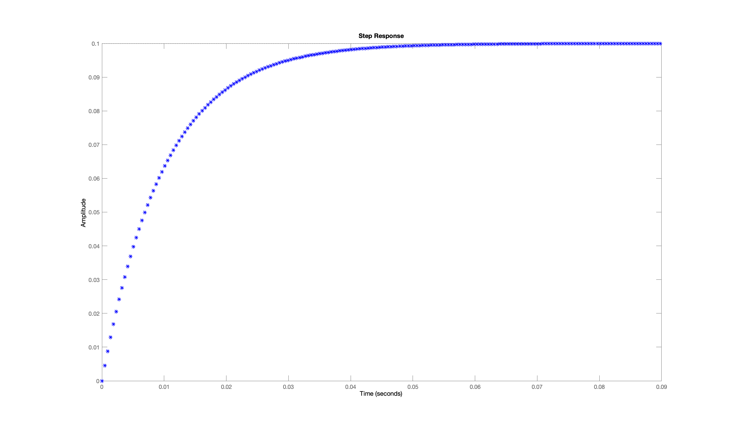
A plot of the step response for b = 10 and \lambda = -100 is given below. Note that the step response settles to \frac{b}{-\lambda} as t \rightarrow \infty, and has risen to about two-thirds of the steady-state at t \approx \frac{1}{-\lambda}.
What happens if x(t) = u(t-t_0)? If y(0) = 0 and x(t) = 0 for t \lt t_0, then y(t) = 0 for t \lt t_0 and
If we want to move the crane to positions other than the beacon position at d=0, we will need to specify a desired position along the track. The desired position, which we will denote as d_{in}(t), will become an input to our position controller, which will try to keep the drane position, d(t), close to the desired position d_{in}(t).
A proportional feedback approach to controlling the crane's position would be to make the crane velocity proportional to the difference between the desired and measured crane positions, as diagrammed for the DT case in the figure above. Then the velocity is given by
In order to determine how the performance of this proportional-feedback controller changes with as we increase or decrease gain, we substitute the control formula in to the distance-velocity relation for the crane,
If $d(0) = 5$ meters, and $d_{in}(t) = 1$, what is the exact solution for $d(t)$ as a function of $K_p$?
We will continue our investigation first-order systems with inputs, but switch to the context of operational amplifiers.