Lead Compensation
Please Log In for full access to the web site.
Note that this link will take you to an external site (https://shimmer.mit.edu) to authenticate, and then you will be redirected back to this page.
What follows is a very brief discussion of lead compensators, with some short questions interspersed. We are trying to give you the "why is this useful" and and the "how to design with it" ideas first, before the formal theory (based on Nyquist diagrams).
We have usually divided the forward path of our archetype feedback system in to the controller (what we design), with transfer function K(s) , and the "plant" (what we are controlling), with transfer function H(s). We will deviate slightly from the K(s) and H(s) notation, and further divide the controller in to the product of a constant gain K, and a normalized compensator transfer function, H_c(s). In this way, candidate compensators can be more easily compared. A good compensator is not the one with the highest innate gain, but the one that, after optimizing over K, yields a feedback system with the smallest tracking errors and highest disturbance rejection.
In addition, for brevity, when we are referring to the closed-loop transfer function, we will denote it as G(s), where G(s) is given by what should be the comfortably-familiar Black's formula:
When we refer to characterizing or analyzing a system by plots of its frequency response, like the magnitude and angle plots that comprise Bode diagrams, we are NOT referring to the generalized notion of frequency, denoted by the complex variable s. Rather, we are using frequency response to mean the response to sinusoidal excitations over a range of repetition periods. More specifically, suppose we are given that in open-loop,
If a system is stable, we can measure the frequency response by applying unit amplitude sinusoidals, waiting until the output achieves sinusoidal steady state, and measuring the amplitude and phase shift of the output. Even if a system is not stable, the above construction can be evaluated mathematically, just not measured practically.
What happens if the denominator in the expression for the closed-loop frequency response,
In fact, K H_c(j \omega_0 ) H(j \omega_0) need only be close to -1 to cause problems, and the closer it is to -1, the further G(j\omega_0) will be from unity. One can make a more formal link to closed-loop stability, but for now, it is sufficient to note that IT IS BAD FOR
For K H_c(j \omega_0 ) H(j \omega_0) to equal -1, an angle and a magnitude condition must each be satisfied:
-
Magnitude condition: |K H_c(j \omega_0 ) H(j \omega_0)| must be equal to 1.
-
Angle Condition: \angle \left( K H_c(j \omega_0 ) H(j \omega_0) \right) must equal +\pi or - \pi radians or +180 or - 180 degrees.
Since being exactly equal to -1 is unlikely, but being near is also bad, we need to define metrics for how close we are to the dreaded -1. To that end, there are three terms commonly used to describe the closeness:
-
Unity gain frequency ( \omega_{unity}): the value of \omega such that |K H_c(j \omega_{unity} ) H(j \omega_{unity})| = 1 . It is possible to have multiple unity gain frequencies, though it is uncommon.
-
Phase Margin : How far of \angle \left(K H_c(j \omega_{unity} ) H(j \omega_{unity})\right) is from - \pi or +\pi radians or +180 or - 180 degrees when the magnitude is unity. Phase margin is usually specified in degrees, and is (in degrees):
- Gain Margin : For those values of \omega for which
\angle \left(K H_c(j \omega ) H(j \omega)\right) equals either
+180 or - 180, the gain margin (in dB) is defined as
-1 times the least positive 20 log |(K H_c(j \omega ) H(j \omega))|.
If the gain margin is negative, then
|(K H_c(j \omega ) H(j \omega))| > 1for all \omega's for which the phase is 180 degrees.
Phase and gain margins can be positive or negative, but they are only guaranteed to indicate a problem when they are close to zero. To better understand what we mean by "problem", consider the three-pole example in the next section.
Consider the three-pole example
Consider the open-loop margin plot and the closed-loop step response for the cases K = 5, K=20 and K=50 below. As is clear from the plots, the phase margin decreases with higher and higher gains (values of K), and the step response becomes more oscillatory. The low phase margin was a correct indication of a problem, as the oscillation in the step response at K=50 is certainly a problem.
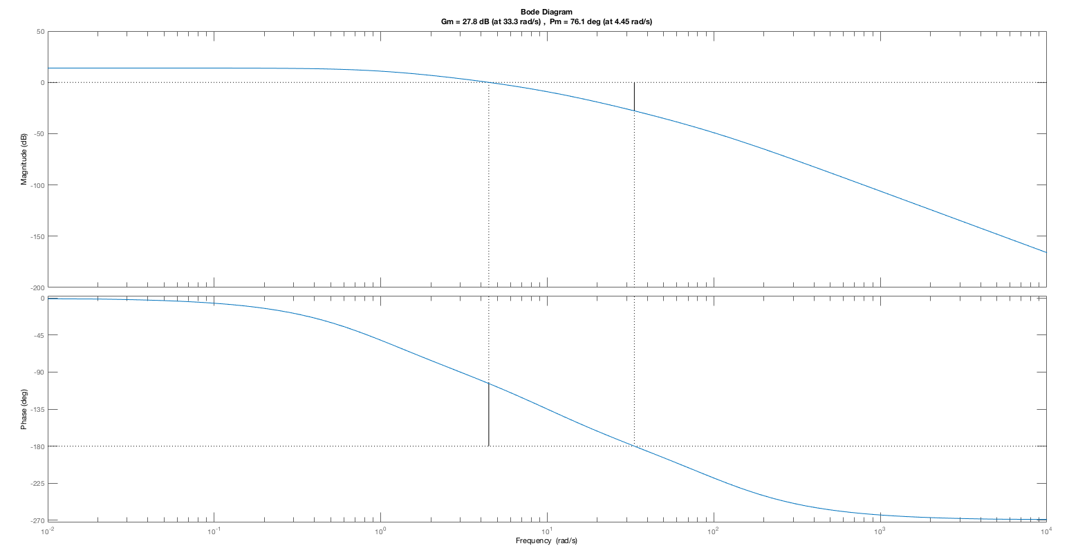
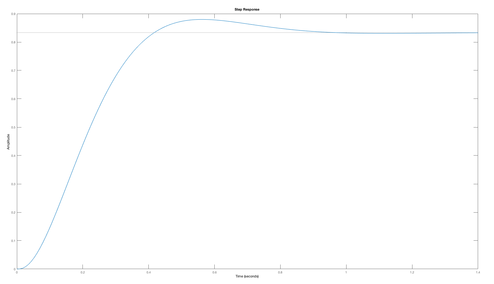
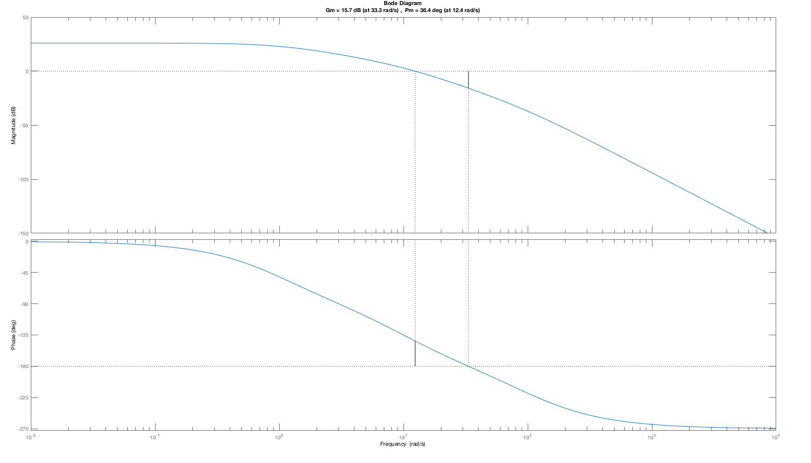
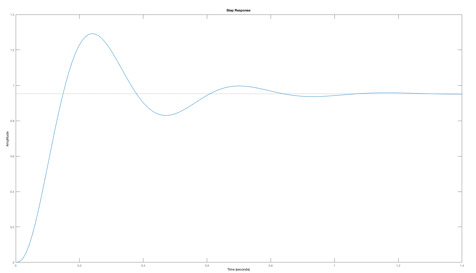
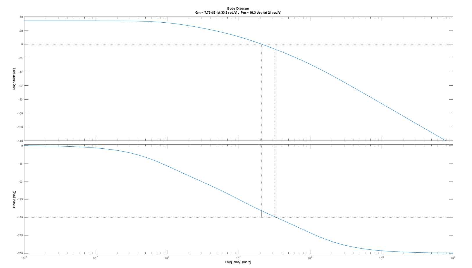
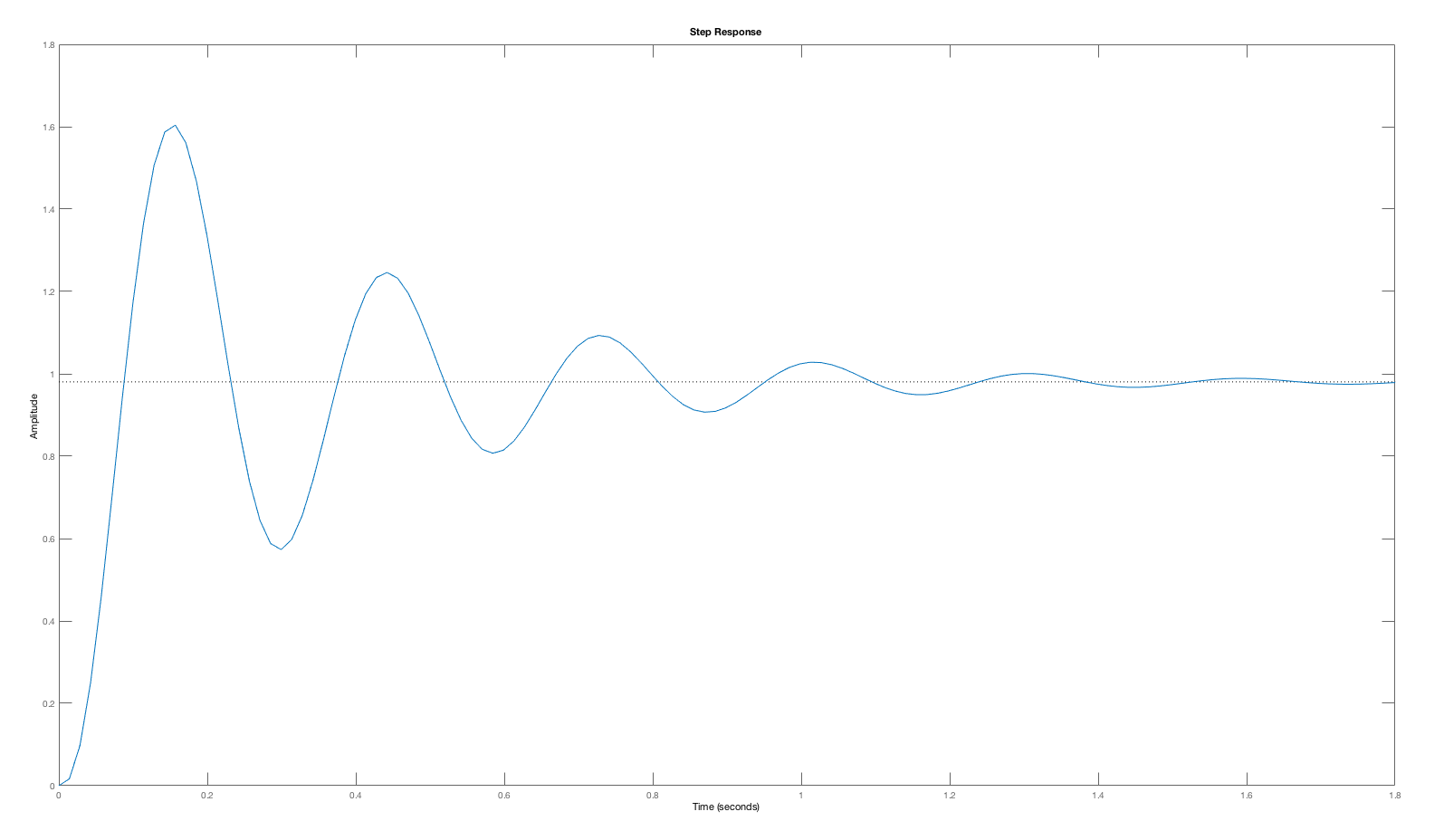
One might expect that an open-loop system with a small phase margin will likely result in a closed-loop system with an oscillatory step response, such as the particularly pronounced K = 50 case. But phase- margin-based predictions are not quantitative. The oscillation amplitude of a closed-loop system, including its oscillation frequency, is far more readily predicted by considering the Bode plot for the closed-loop system with K=50 (see figure below). As the Bode plot for the closed loop system shows, the frequency response has a large peak, exactly at the frequency of the oscillating step response. Or, we could have considered the root-locus plot for this system, which would have indicated that at K=50, the poles of the closed-loop system move close to the imaginary axis (the second figure below). Finally, when K=5, the gain is too low to accurately track the input, and the steady state value for the step response (which should be one) is off by more than ten percent. Phase and gain margin tell us little about this low gain problem.
So, why bother with gain and phase margin?
 Bode Plot of the CLOSED-LOOP response for the $K=50$ case, showing
the peaking of the response at $\approx 22$ radians/second.
Bode Plot of the CLOSED-LOOP response for the $K=50$ case, showing
the peaking of the response at $\approx 22$ radians/second.
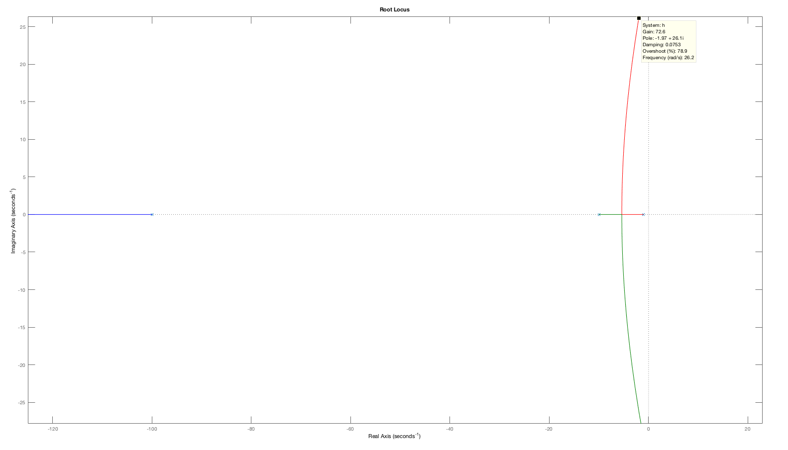 The root-locus plot for $H(s) = \frac{1000}{(s+1)(s+10)(s+100)} $,
showing a pair of poles moving towards the imaginary axis as the
gain increases (the highest gain shown is $K \approx 70$).
The root-locus plot for $H(s) = \frac{1000}{(s+1)(s+10)(s+100)} $,
showing a pair of poles moving towards the imaginary axis as the
gain increases (the highest gain shown is $K \approx 70$).
We know that a small phase margin is bad, but as noted above, we have other tools that can provide a far more sophisticated analysis of the kinds of problems indicated by a low phase margin. On the other hand, if we do have low phase margin, there is an easy way to design a compensator to increase it.
The key insight to increasing phase margin is that the angle for a product of two transfers functions is the sum of the two angles. That is,
To see how to use this additive property, suppose K H(s) has a small phase margin. For systems dominated by poles (as most physical systems are), the angle of the frequency response will be negative. Then since the phase margin is small, the angle at unity gain must be close to -\pi, or in degrees,
But not so fast! We can not exactly enforce the unit magnitude constraint, while still adding phase, but we can come close. And, we can come close with a transfer function that is easily implemented using an operational amplifier, a few resistors, and a capacitor.
Consider the normalized compensator transfer function:
What is magnitude of the normalized compensator at zero frequency?

In terms of p and z, what is the magnitude of the compensator in the limit as \omega \rightarrow \infty?
Can we use this zero-over-pole compensator to add phase at the unity gain frequency? And can we come close to keeping the magnitude of the compensator near one, so we do not shift the unity gain frequency?
Consider the example of a compensator whose zero is z = -10, and whose pole is p = -100. With this pole and zero, the resulting compensator is of the form
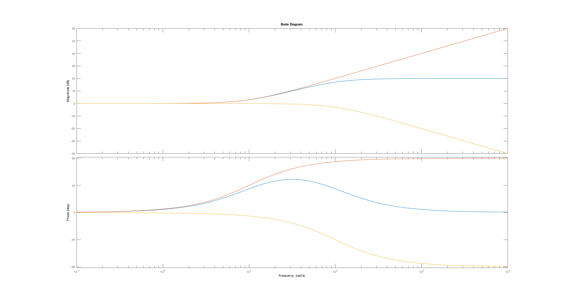
In the figure below, there are three plots. One is a plot of H_c(s), whose magnitude is level, and then monotonically increases, before leveling off a factor of ten higher. Its angle increases, but visually, it seems to start increasing at a lower frequency than its magnitude increases. Perhaps we can use this to approximate our ideal phase margin increaser.
Overall, the angle of the compensator rises from an angle of 0, achieves a maximum, and then returns to an angle of 0. We also show the seperate components in the plot below. There is the angle and magnitude for just the numerator zero, which is flat until the zero frequency and then the angle and magnitude increase monotonically. The is also the angle and magnitude for the denominator pole, which is also flat until the pole frequency, and then starts monotonically decreasing in angle and magnitude.
NOTE: we refer to this compensator as a LEAD compensator because the zero leads the pole.
Suppose H_c(s) = \frac{p}{z} \left(\frac{s-z}{s-p} \right) , with real z, p < 0. In terms of p and z, what is the value of \omega_{extreme} , the frequency where the angle of H_c(j \omega ) achieves its extreme (either maximum or minimum)? Hint: recall that the angle of H_c is the angle of the zero minus the angle of the pole. Differentiate the difference with respect to \omega , and find where the derivative is zero.
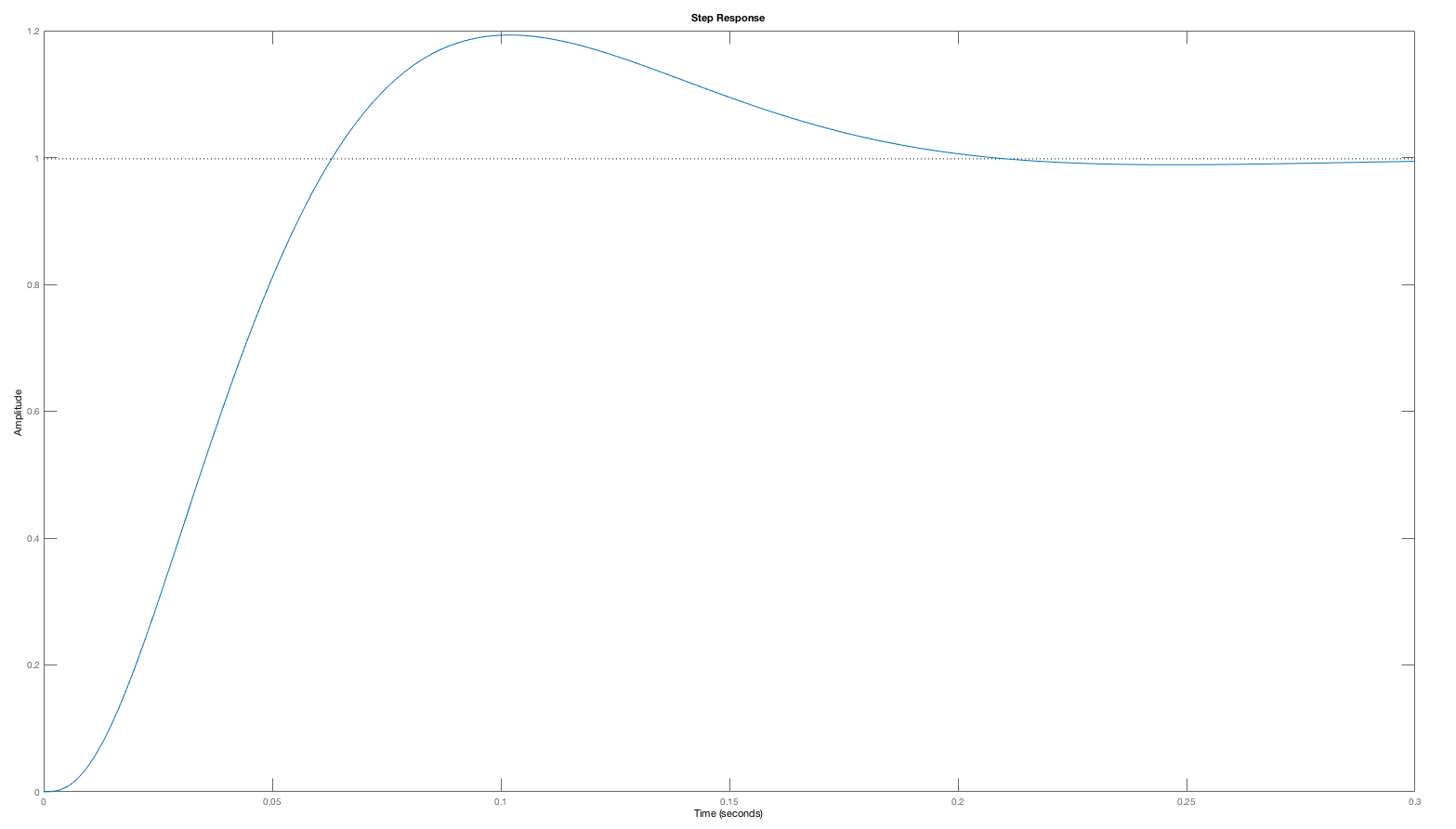
Let us return to the worst example from above, H(s) = \frac{1000}{(s+1)(s+10)(s+100)} with K = 50. The phase margin is quite low, roughly 15 degrees, and the step response oscillates. Suppose we place a normalized compensator with a zero at approximately the unity gain frequency ( z = -20 ) and a pole at a ten times higher frequency (p = -200)? What is the new phase margin (you will need a bode plotter, use either matlab or python). To check yourself, we have plotted the step response of the compensated system (which is QUITE an improvement).
Let us try an example from an earlier lab: the transfer function for the copter arm. Recall that when we included the thrust-buildup pole (that p_c pole value), the transfer function was approximately
Is there any K for which KH(s) has a positive phase margin?
Suppose we have three possible compensators:
H_D if H_D(s) were a compensator you could
pick.
Does using H_C(s) give you a postive phase margin?
Does using 10 \frac{s+ 10 \beta}{s + 100 \beta} , give you a postive phase margin for any \beta > 1? (Hint: with \beta > 1, the leading zero in the compensator is more negative than the most negative pole in the plant).
In a lead compensator, the zero "leads" the pole. That is, the compensator's zero is less negative than the compensator's pole. Which of the following statements about lead compensators is true?
"If a lead compensator is applied to a stable three real pole system, and the compensator's zero is as negative, or more negative, than the most negative system pole, then the compensator will NOT improve the system's phase margin."
Hint: What about H(s) = \frac{60}{(s+1)*(s+2)*(s+3)}?
"If a lead compensator is applied to a system with one negative real pole and two poles at 0, and the compensator's zero is as negative, or more negative, than the most negative system pole, then the compensated system will NEVER have a positive phase margin."