Model Parameters

Parameter Derivation

% Parameters
Ke = 5.5e-3;  % back-emf per radian/sec motor rotational velocity
Km = 5.5e-3;  % Torque per amp
Jm = 3e-6;  % Motor moment of inertia
Ja = 4.5e-4; % Arm moment of inertia
Rm = 1;      % Motor resistance
Rs = 1;      % Series resistance
La = 0.15;   % Arm length in meters
Kf = 10e-6;  % Motor Friction
Kt = 1.8e-3; %Torque coefficient for arm.

At the top of the code for the last few weeks, we've been including a list of system parameters with actual values such as moments of inertia, How did we come up with some of these parameters?

We approximated the moment of inertia of the propeller J_m as that of a flat rod rotating around its center. This moment is expressed using this equation:

In the case of our propeller it works out to be:

We approximated the moment of inertia of our arm assembly as that of a narrow rod on an axis and a point mass summed together. Therefore:

Based on our measurements we got a value of about J_a = 4.5\times 10^{-4} \text{kg}\cdot \text{m}^2.

Motor Coefficients

We calculated a number of motor parameters through a series of experiments briefly detailed below. I'm including a writeup on how we did this in case you want to do something similar (don't feel obligated) for this setup or in the context of other systems!:

Thrust Coefficient

We first mounted the propeller assembly on a scale and zeroed the weight when it was not running like shown below. We then proceeded to gradually increase the voltage applied to the motor while tracking the current through the motor as well as the change in sensed mass on the scale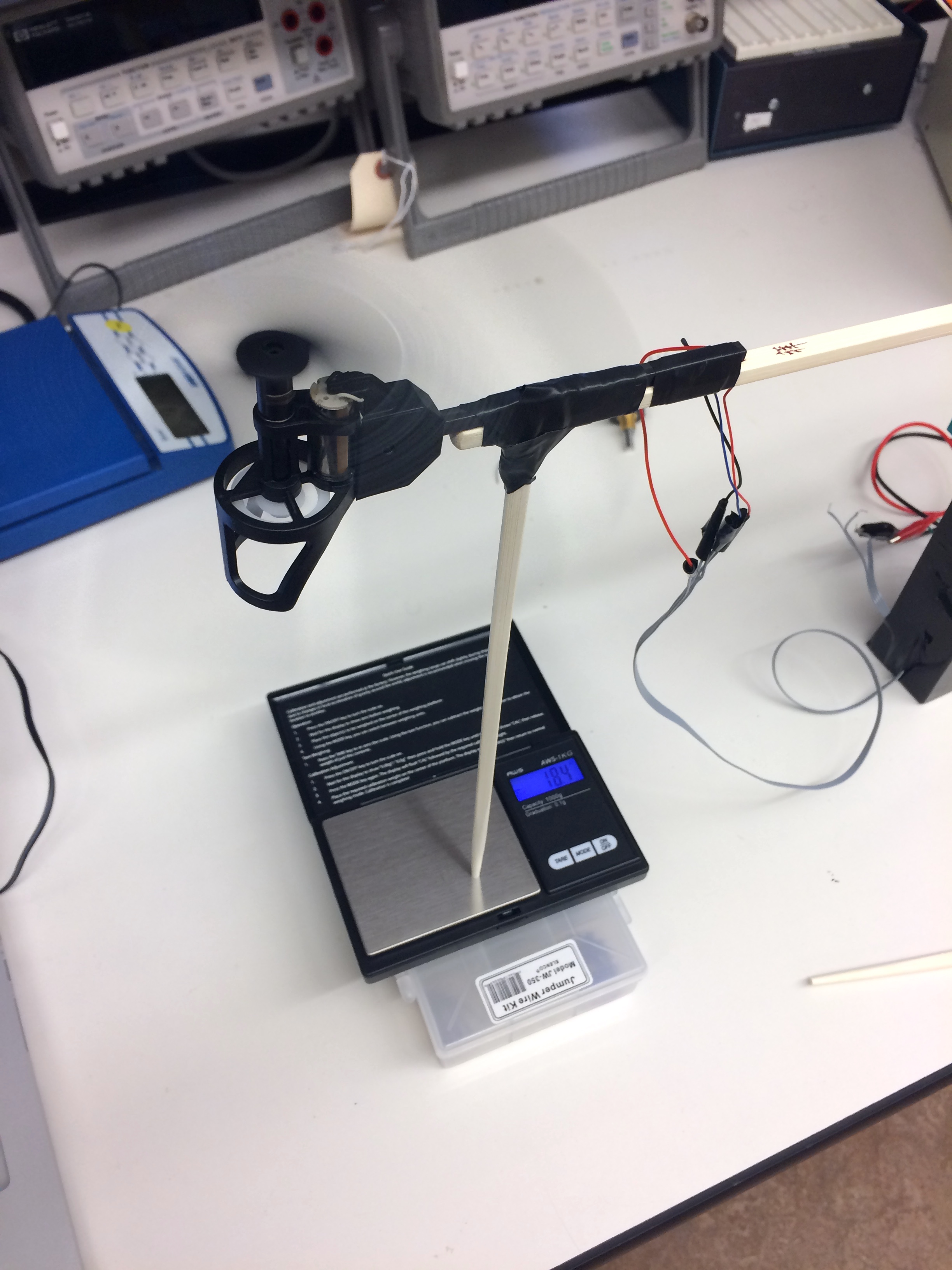 We could use the readings from the scale to extract measurements of thrust based on voltage, current, and ultimately back EMF. For example, if the scale began reading "-2.5g" that would correspond to an equivalent force of $0.0025\text{ kg}\cdot 9.81\text{m}\cdot\text{s}^{-2}=0.02454 \text{N}$.

Motor Coil Resistance

The motor's electrical resistance R_m was measured in two ways. First we just took an Ohmmeter and attached read the resistance. Additionally, we found a slightly different value by incorporating the motor into a circuit with a number of other low-value fixed resistors, and then by measuring the voltage drop across parts of the circuit could back out a value of approximately R_m\approx 1.0\Omega.

Motor Speed and Back EMF

The Back EMF of the motor was relatively easy to calculate once we had a resistor value R_m to work with. What was trickier to do was determine the back EMF coefficient K_e. For that we need to know the motor's angular velocity \omega_m as a function of current or voltage or something and we figured that out by building a cheap phototransistor-based (Digikey part number 1080-1152-ND in case you're interested) optical sense-circuit placed immediately below the propeller while it was running. By monitoring the output of this simple circuit on an oscilloscope we could use the deviation in signal (generated by room light being "chopped" by the rapidly passing propeller blade) to get real time measurements of the motor speed.

The system in action looked like the following:

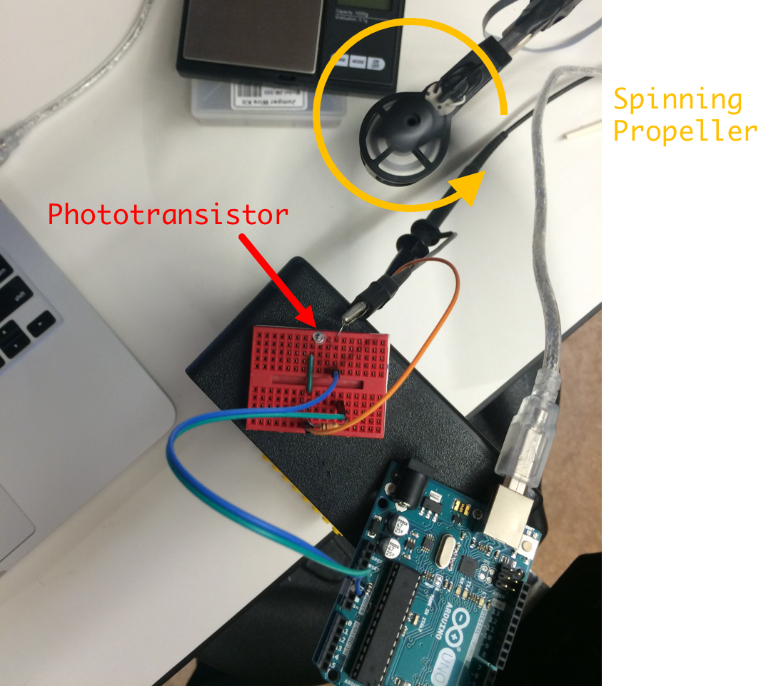
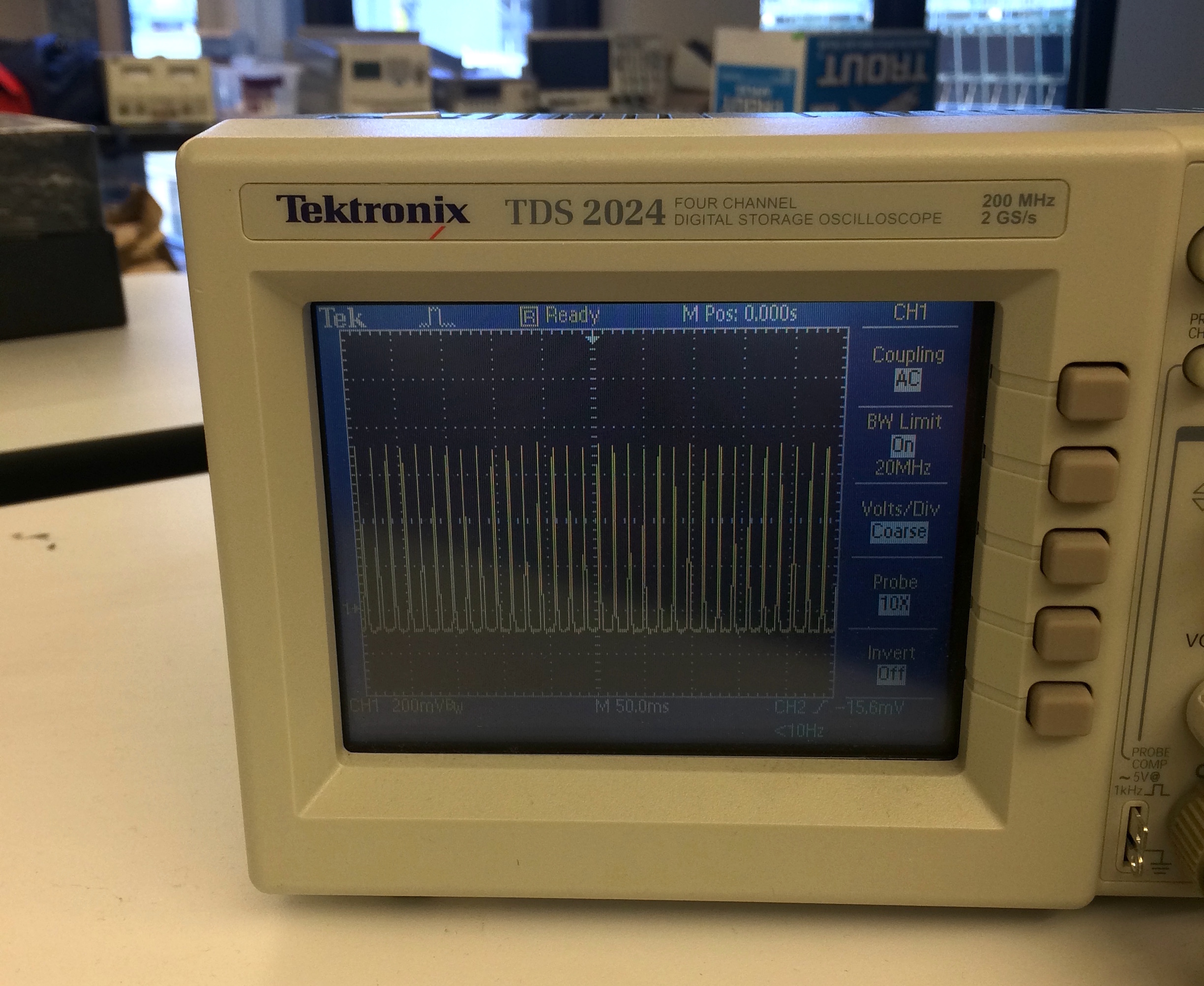
And the output signal in real-time looked something like this. Note we weren't concerned so much with the amplitude of our signal here, instead just the periodicity of the deviations (two "blips" per revolution...one for each blade)

Numbers...

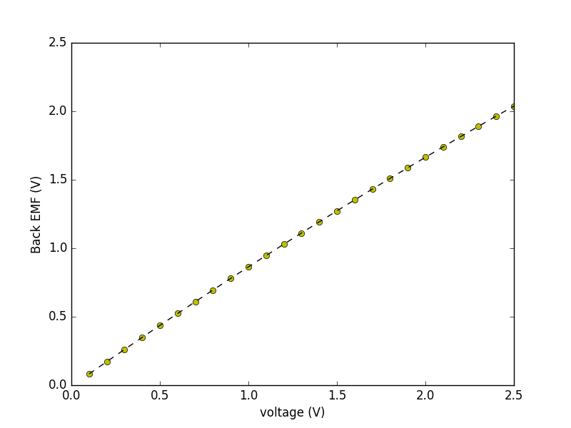
With data collected we could start coming up with relationships between parameters measured. We found the relationship between the motor voltage and the current through the motor to be roughly quadratic in shape (data points are yellow dots and fitted curve is black dashed line):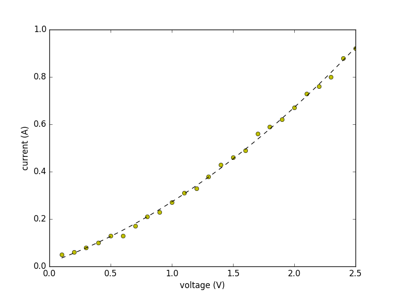 In particular, current as a function of applied voltage was found to be: $$ i\left(v\right) = 0.071v^2 + 0.19v + 0.01619 $$ where $i$ is in Amps and $v$ is in volts. (Note these readings were in steady state).

Since we already had a rough idea of the coil resistance (R_m \approx 1.0\Omega), we could use this curve to come up with an expression for the back EMF as a function of applied voltage by saying (review our simplified motor model from week 1):

When we plot our fitted function using this modifiation we end up with the following new fitted equation:

Which fits very nicely to a first order expresion: $$ v_{emf}\left(v\right) \approx 0.91v - 0.0081 $$ So this is saying that back EMF is roughly linearly proportional to voltage applied to the motor. Now we need to figure out if our relationship between back EMF and propeller speed $\omega_m$ is linear. To do this we can plot data points of calculated back EMF (figured out above) for a given voltage compared to measured propeller speed for that same given voltage. When we do this we get the following plot (data in yellow, fitted curve in black dashed): And when we fit those yellow data points to a first order function we get the following: $$ v_{emf}\left(\omega_m\right) \approx 0.0053\omega_m - 0.09381 $$ Ignoring the offset this is saying: $$ v_{emf} = 0.0053\omega_m $$ and since $v_{emf} = K_e\omega_m$ we can now say that $K_e \approx 0.0053 \text{V}\cdot\text{rad}\cdot\text{s}^{-1}$!

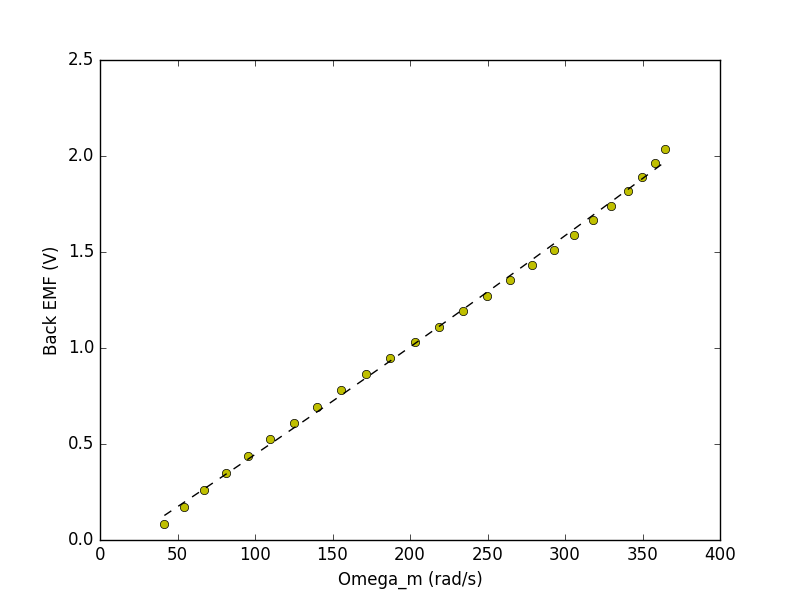
We also made the assumption that the back emf coefficient (K_e) is equal to the motor torque coefficient K_m, which is often done for motors so K_m = 0.0053 as well!

The last critical term that we're missing is the relationship between motor speed \omega_m and the thrust generated by the propeller. We expect this thrust to be proportional to the square of our motor speed and when we plot those two values out we get the following set of data points (yellow):

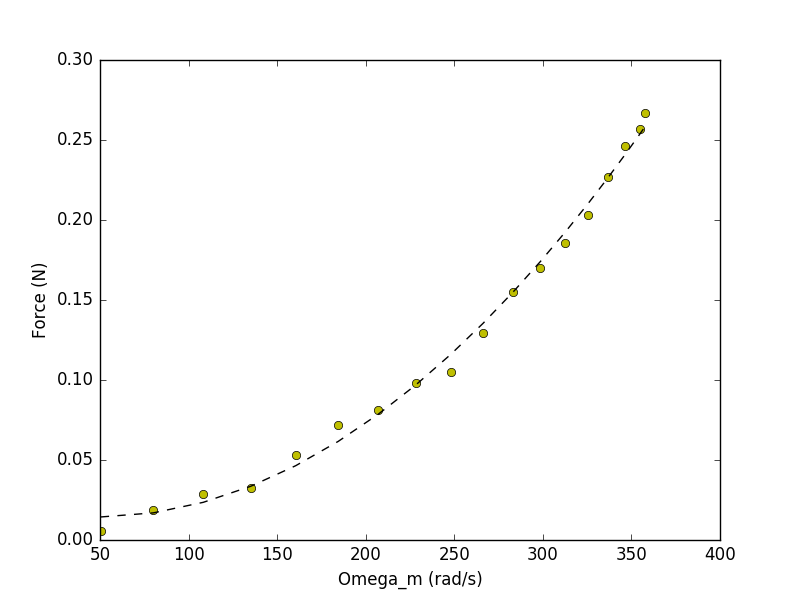
Fitting this to a second order function yields the following where force/thrust is in Newtons.

This is very quadratic as we expected, and going back to our earlier model derivation in week 1, we're going to need to linearize around our usual point of operation to turn this into something that we can fit into our LTI (Linear Time-Invariant) model. If we linearize around when \omega_m\approx 300 \text{rad}\cdot\text{s}^{-1} we'll get:

Which is then:

With this number we can then say that the "deviation" in force around our operating point can be approximated with the expression:

OK we have some parameters!