Eigenvalues to LQR

For convenience, we are repeating all of the pre-prelab's L-motor-driven arm question (other than the actual questions boxes, of course). We are revisiting the example and using LQR to design its controller.

Show/Hide

An L-Motor-Driven Arm

In this problem set, we will consider a problem that is similar to the propeller-levitated arm, a lego-motor-driven arm (for brievity, an Lmotor-driven arm). The similarities will make it easier for us to understand the structure of this new control problem, but differences will all us to raise additional issues, while also giving us a chance to practice with the state-space concepts.

In earlier versions of 6.302, we rotated a heavier arm using a geared Lego motor, shown in the figure below. The figure also shows that we used two rubber bands to create an angle dependent torque on the motor (both to assist the motor when holding heavy loads, and to eliminate gear "backlash"). That angle dependent force will have a number of interesting consequences, ones that we hope will help you develop a better understanding of controller design.

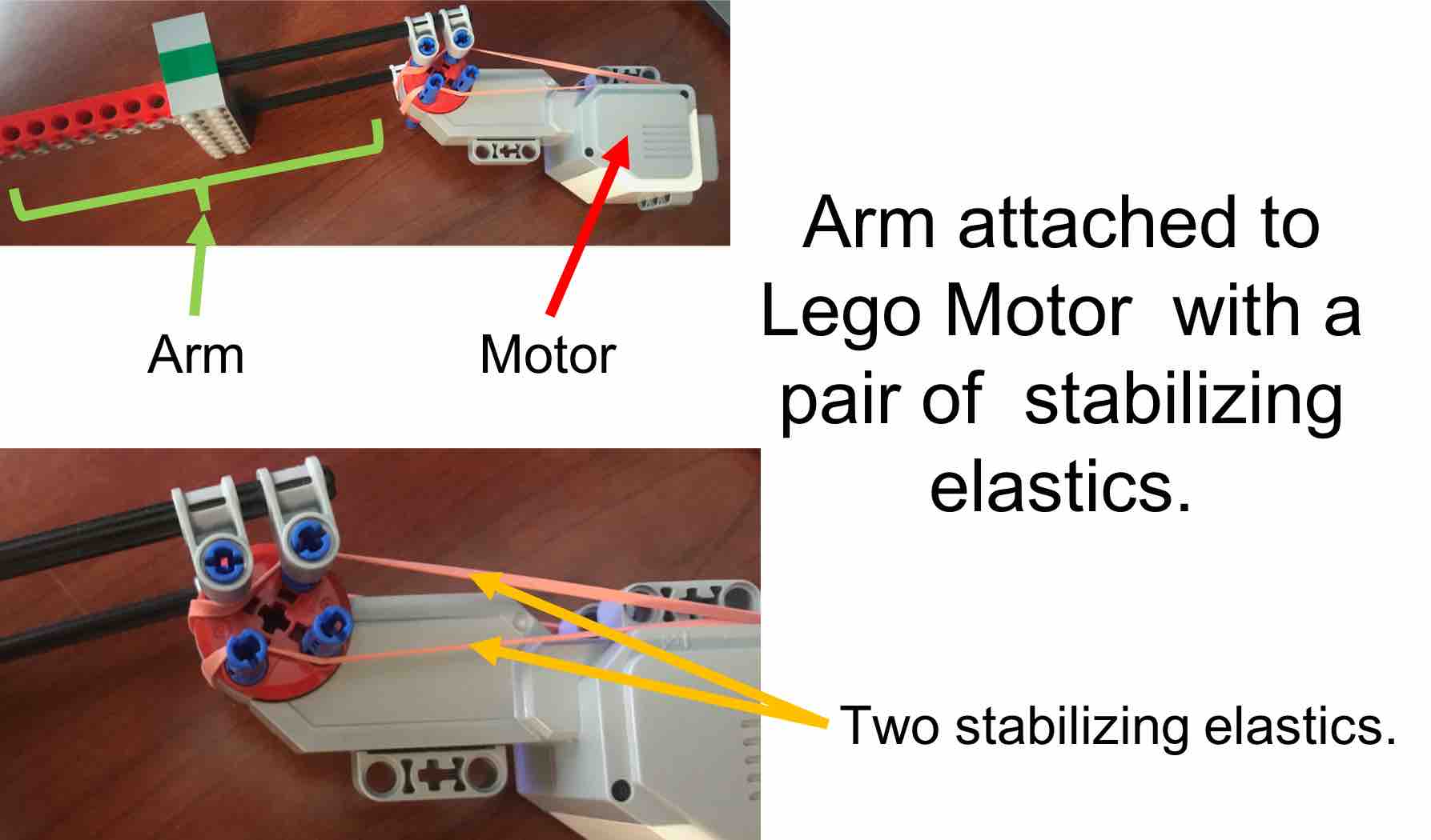
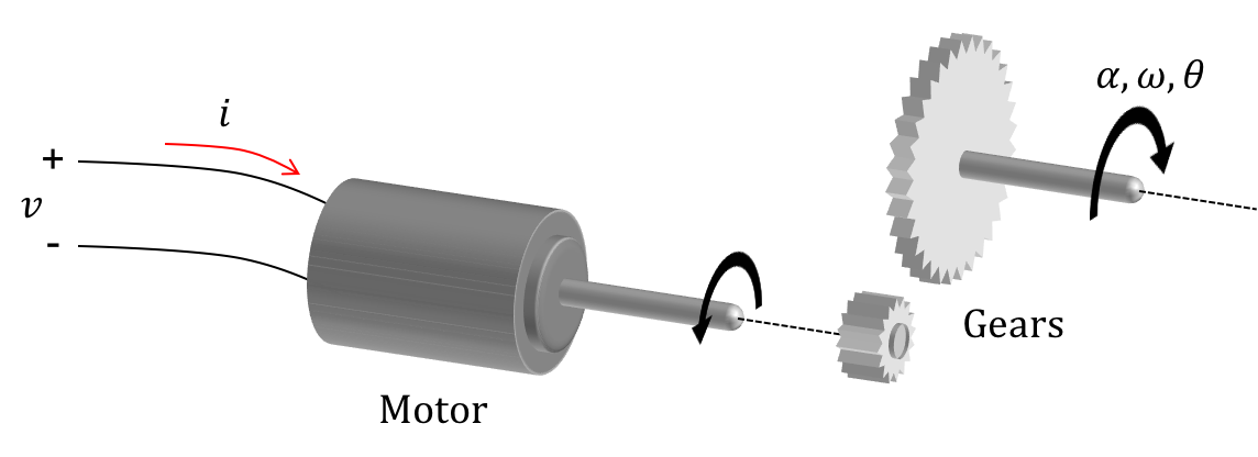
The L-motor is a geared brushed motor, just like the propeller motor. By changing the motor voltage, v, we change the motor current, i_m, which is proportional to the torque generated by the motor. The net arm torque, a sum of motor-, gravity-, and elastic-generated torques, results in an arm rotation characterized angular acceleration, \alpha, and angular velocity, \omega, and rotation angle \theta, as shown in the figure below.

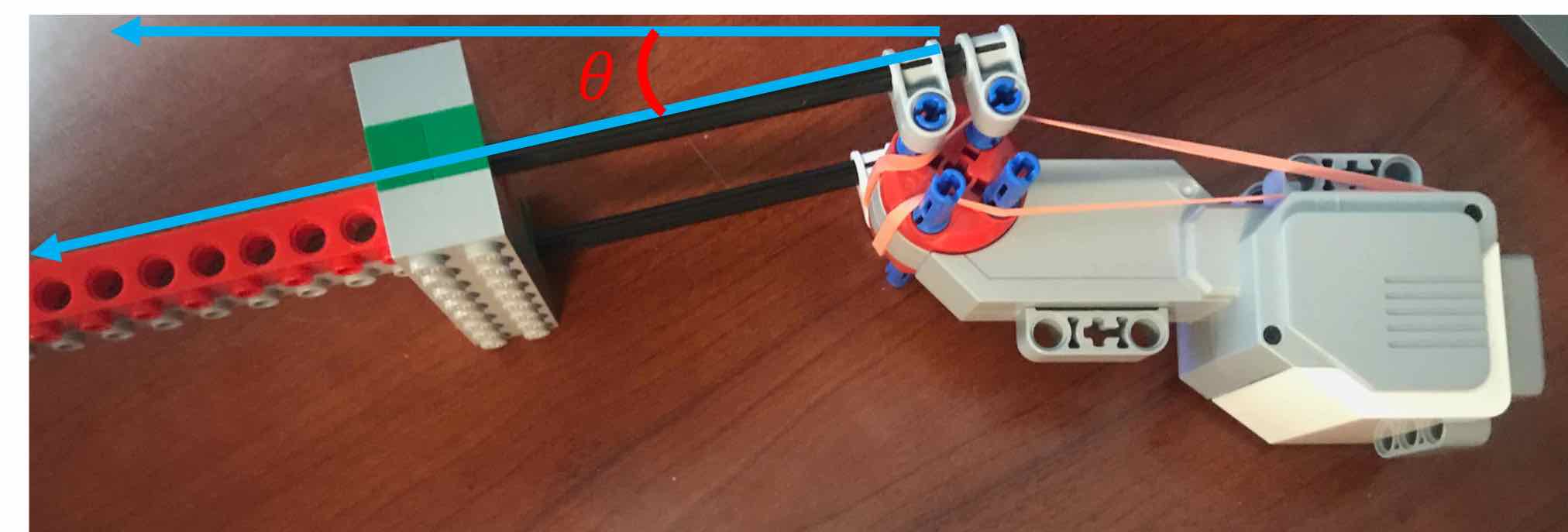
We can sense the Lmotor-driven arm angle using the same kind of angle sensor we use for the propeller arm, by linking the shaft of the angle sensor to the shaft of the motor (using heat-shrink tubing actually). As an example, using our angle sensor, we could easily meaure the \theta in the figure below as approximately \frac{-\pi}{6}.

In fact, we can reuse most of our propeller-levitated arm hardware in an Lmotor-driven arm controller, since they both use brushed DC motors. We can use the same angle sensor, and we can drive the Lmotor using the same H-bridge (the Pololu board) with almost the same PWM voltages (though lego motors are designed to work with lower-frequency PWM signals). In fact, we could even use exactly the same PID controller, though we might find that good K_i, K_d, and K_p values for the Lmotor-driven arm will be different from good values for the propeller arm.

The issues in designing state-space controllers are a little different, however, as we shall see.

Generating a State-Space model

We will need a few physical relationships in order to derive a state-space model, but thankfully, the Lmotor-driven arm model does not require linearization.

The physical relationships

As in the propeller-levitated arm, the Lmotor-driven arm angle, \theta(t), is related to its angular velocity, \omega(t), through differentiation,

\frac{d \theta}{dt} = \omega(t),

and of course, the angular velocity of the arm is related to arm angular acceleration through differentiation,

\frac{d \omega(t)}{dt} = \alpha(t).

The product of the arm's moment of inertia, J, and its angular acceleration, \alpha, is equal to the torque on the arm \tau,

J \alpha(t)=\tau(t) = \tau_m(t) + \tau_b(t) + \tau_f(t),

where \tau_m is the motor-generated torque, \tau_b is the net torque generated by the rubber bands, and \tau_f is the torque due to friction. We are going to assume the arm is rotating parallel to the ground, so that we can ignore gravity as a source of torque on the arm.

As we have seen before, motor torque, \tau_m, is proportional to motor current,

\tau_m = K_m i_m,

where i_m is the motor current and K_m is the current to torque conversion factor. We can model the net torque generated by the two rubber bands as proportional to arm angle, as long as the bands have been placed so that their forces balance at \theta =0. If so, then

\tau_b = K_b \theta,

where \tau_b is the net elastic torque and K_b is the proportionality constant. Finally, the friction torque can be modeled as proportional to angular velocity,

\tau_f = -K_f \omega,

where K_f is the friction coefficient, and the negative sign is because the friction force always acts to oppose motion.

Since the Lmotor is a brushed motor, we can model it in the same way we modeled the propeller motor. That is, we can use a circuit model to relate the voltage across the motor to the current through the motor, and after scaling by K_m, relate the motor voltage to the motor torque. If we model the motor as a series combination of a motor coil resistor, R_m, a motor coil inductor, L_m, and a rotational-velocity dependent voltage source, v_{emf}, the current through the motor, i_m, can be related to the drive voltage, v, by

v(t) = R_m i_m(t) + L_m\frac{di_m(t)}{dt} + v_{emf}(t).

The motor's inductance and resistance are much larger in the propeller motor, so the above relation can not be simplified. Further, we know from earlier labs that the v_{emf} is proportional to the motor speed, \omega_m,

v_{emf}(t) = K_e\omega(t).

Values for the physical parameters.

(http://nxt-unroller.blogspot.com/2015/03/mathematical-model-of-lego-ev3-motor.html)

L_m = 0.005 is the motor inductance in Henries.

J = 0.0015 is the arm-plus-motor moment of inertia.

R_m = 7.0 is the motor's series resistance in ohms.

K_e = 0.46 is the back-emf per radian/sec of motor rotational velocity.

K_m = 0.3 is the torque per ampere of current.

K_f = 0.00073 is the torque due to friction per radian/second.

K_b = 0.0 \;or\; -0.1 is the elastic torque per radian (due to the rubber bands) and is negative because the elastic was used to oppose arm motion.

Generating the State-Space Matrices

We can describe our Lmotor-driven arm, our "plant", as a single-input single -output (SISO) state-space system with the motor voltage as the input and the arm angle as the output. The generic form of the state-space model using \textbf{E}, \textbf{A}, \textbf{B}, and \textbf{C} matrices is

\textbf{E} \frac{d}{dt} \textbf{x} = \textbf{A}\textbf{x}(t) + \textbf{B} u(t)

and

y(t) = \textbf{C} \textbf{x}(t),

where the states in the system (there are three) are the elements of the three-length vector, \textbf{x}, u is the motor voltage, and y is arm angle.

There are an infinite number of state-space models that can be generated from our physical model of the Lmotor-driven arm, even though we have specified the input and output. To make it easier to grade, we will constrain which element of the vector \textbf{x} goes with which physical state by fixing the input and output matrices, \textbf{B} and \textbf{C},

\textbf{B} = \begin{bmatrix} 1 \\ 0 \\ 0 \end{bmatrix}

\textbf{C} = \begin{bmatrix} 0 \ 0 \ 1\end{bmatrix}.

Unfortunately, there are so many zeros in \textbf{B} and \textbf{C} that the state-space system is still not unique, so we will also constrain the \textbf{E} to be diagonal, with diagonal entries L_m, J, and 1.

What is the state-space matrix \textbf{A} for our Lmotor driven arm, assuming that there are rubber bands? Please enter the \textbf{A} matrix below, and remember to use Python form, so, for example, the \textbf{E} matrix would be specified as

`[[5.0e-3, 0, 0], [0, 1.5e-3,0],[0, 0, 1]]'

Poles and Eigenvalues.

In the SISO state-space system, the transfer function from plant input u to plant output y is given by

H_{plant}(s) = \textbf{C} \left(s\textbf{E} - \textbf{A}\right)^{-1} \textbf{B},

but how does that formula relate to the transfer functions from classical control. For example, how do we relate the above matrix formula to an L-zero, N-pole transfer function,

H(s) = \frac{(s - z_1)(s-z_2)...(s-z_{L-1})(s-z_L)}{(s - p_1)(s-p_2)...(s-p_{N-1})(s-p_N)},

which, if the poles are distinct, can be expanded in to

H(s) = \frac{\alpha_1}{s - p_1} + \frac{\alpha_2}{s - p_2} + ... + \frac{\alpha_N}{s - p_N}.

Let us start with the \textbf{E} = \textbf{I} (the identity matrix) case. In this case, the eigenvalues of \textbf{A} are the poles of H(s) Recall that if \lambda_i is an eigenvalue of \textbf{A}, and \textbf{V}_i is the associated eigenvector, then

\textbf{A} \textbf{V}_i = \lambda_i \textbf{V}_i.

If there are no repeated eigenvalues, that is the eigenvalues are distinct, then

\textbf{A} \begin{bmatrix} \textbf{V}_1 \textbf{V}_2 ... \textbf{V}_N \end{bmatrix} = \begin{bmatrix} \textbf{V}_1 \textbf{V}_2 ... \textbf{V}_N \end{bmatrix} \begin{bmatrix} \lambda_1 \ 0 \ ... \ ... \ 0\\ 0 \ \lambda_2 \ 0 \ ... \ 0 \\ ... \ ... \ ... \ ... \ ...\\ 0 \ ... \ ... \ 0 \ \lambda_N \end{bmatrix},

or

\textbf{A} \textbf{V} = \textbf{V} \Lambda

where \textbf{V} is a matrix of eigenvectors. The columns of \textbf{V} are the eigenvectors of \textbf{A}, and are guaranteed to be linearly independent if \textbf{A}'s eigenvalues are distinct, and therefore \textbf{V} will be invertible. Then using the inverse of \textbf{V},

\textbf{V}^{-1} \textbf{A} \textbf{V} = \Lambda,

and we say that the eigenvectors diagonalize \textbf{A}.

Consider a change of variables, in which the vector \textbf{x} is written as a weighted combination of the eigenvectors of \textbf{A} (also known as \textbf{x}'s spectral decomposition),

\textbf{x}(t) = \textbf{V} \textbf{w}(t)

where \textbf{w} is the vector of eigenvector weights. Using this change of variables in the state-space model,

\frac{d}{dt} \textbf{V} \textbf{w}(t) = \textbf{A}\textbf{V} \textbf{w}(t) + \textbf{B} u(t),

and

y(t) = \textbf{C} \textbf{V} \textbf{w}(t).

If we then multiply by \textbf{V}^{-1}, and define \tilde{\textbf{B}} and \tilde{\textbf{C}} in the new variables,

\frac{d}{dt} \textbf{w}(t) = \textbf{V}^{-1} \textbf{A}\textbf{V} \textbf{w}(t) + \textbf{V}^{-1}\textbf{B} u(t) =\begin{bmatrix} \lambda_1 \ 0 \ ... \ ... \ 0\\ 0 \ \lambda_2 \ 0 \ ... \ 0 \\ ... \ ... \ ... \ ... \ ...\\ 0 \ ... \ ... \ 0 \ \lambda_N \end{bmatrix}, \textbf{w}(t) + \tilde{\textbf{B}} u(t) = \Lambda \textbf{w}(t) + \tilde{\textbf{B}} u(t)

and

y(t) = \textbf{C} \textbf{V} \textbf{w}(t) = \tilde{\textbf{C}} \textbf{w}(t).

where we use the tilde to denote matrices after the change of variables.

Rewriting

H_{plant}(s) = \textbf{C} \left(s\textbf{I} - \textbf{A}\right)^{-1} \textbf{B} = \tilde{\textbf{C}} \begin{bmatrix} \frac{1}{s - \lambda_1} \ 0 \ ... \ ... \ 0\\ 0 \ \frac{1}{s - \lambda_2} \ 0 \ ... \ 0 \\ ... \ ... \ ... \ ... \ ...\\ 0 \ ... \ ... \ 0 \ \frac{1}{s - \lambda_N} \end{bmatrix},\tilde{\textbf{B}}.

If we write out the matrix products and match it to the partial fraction expansion from above,

H(s) = \frac{\tilde{\textbf{C}}_1 \tilde{\textbf{B}}_1}{s - \lambda_1} + \frac{\tilde{\textbf{C}}_2 \tilde{\textbf{B}}_2}{s - \lambda_2} + ... + \frac{\tilde{\textbf{C}}_N \tilde{\textbf{B}}_N}{s - \lambda_N} = \frac{\alpha_1}{s - p_1} + \frac{\alpha_2}{s - p_2} + ... + \frac{\alpha_N}{s - p_N},

we can see that the pole p_i equals the eigenvalue \lambda_i, and the coefficient in the partial fraction expansion, \alpha_i equals the product \tilde{\textbf{C}}_i \tilde{\textbf{B}}_i.

Now consider the case where \textbf{E} is not equal to \textbf{I}, in which case we will make use of generalized eigenvectors and eigenvalues. We say that \lambda_i is a generalized eigenvalue and \textbf{V}_i is the associated generalized eigenvector of the matrix pair \textbf{A},\textbf{E} if

\textbf{A} \textbf{V}_i = \lambda_i \textbf{E} \textbf{V}_i.

and if there are N eigenvalues and eigenvectors, then

\textbf{A} \textbf{V} = \textbf{E} \textbf{V} \Lambda

where \Lambda is the diagonal matrix of eigenvalues and \textbf{V} is the matrix of eigenvectors. The generalized eigenvector and eigenvalue matrices can be computed with matlab's 'eig' command using two input arguments, as in

[V,Lambda] = eig(A,E)

If \textbf{E} matrix is invertible, and the generalized eigenvalues are distinct, we can still use a change of variables to convert the state-space model to

\frac{d}{dt} \textbf{w}(t) = \begin{bmatrix} \lambda_1 \ 0 \ ... \ ... \ 0\\ 0 \ \lambda_2 \ 0 \ ... \ 0 \\ ... \ ... \ ... \ ... \ ...\\ 0 \ ... \ ... \ 0 \ \lambda_N \end{bmatrix} \textbf{w}(t) + \tilde{\textbf{B}} u(t) = \Lambda \textbf{w}(t) + \tilde{\textbf{B}} u(t)

and

y(t) = \tilde{\textbf{C}} \textbf{w}(t).

Poles and transfer functions Beyond E = Identity Assuming \textbf{E} is invertible (but is not necessarily the identity) and that the generalized eigenvalues are distinct, answer the following questions in terms of E, A, B, C, V and L (for \Lambda), and their inverses (e.g. E**-1)

When using state-feedback control

u(t) = K_r r(t) - \textbf{K} \textbf{x}(t)

where r is the reference input. The closed-loop transfer function from reference input to plant output is given by

H_{closedLoop}(s) = \textbf{C} \left(s\textbf{E} - \left(\textbf{A}-\textbf{B}\textbf{K}\right) \right)^{-1} \textbf{B} K_r = \textbf{C} \left(s\textbf{I} - \textbf{E}^{-1}\left(\textbf{A}-\textbf{B}\textbf{K}\right) \right)^{-1} \textbf{E}^{-1}\textbf{B} K_r.

The poles of the closed-loop transfer function are equal to the eigenvalues of what matrix (use A**-1 to denote A^{-1})?

Poles and transfer functions for the Lmotor-driven arm Now use the above formulas (and matlab) to compute the poles and partial fraction expansion representation of the transfer function for the open-loop Lmotor-driven arm plant,

H(s) = \frac{\alpha_1}{s - p_1} + \frac{\alpha_2}{s - p_2} + \frac{\alpha_3}{s - p_3},

which can be reorganized as

H(s) = \frac{\beta_1}{\frac{s}{p_1} - 1} + \frac{\beta_2}{\frac{s}{p_2} - 1} +\frac{\beta_3}{\frac{s}{p_3} - 1},

where \beta_i = \frac{\alpha_i}{p_i}.

Note that one pole is much larger than the other two, and its associated \beta much smaller. That suggests H(s) could be well approximated without that pole, an idea we return to below.

The elastic torque and \( K_r \)

Since you completed the above problem, you know that the states for the system are i_m, \omega, and \theta, in that order. If you want to design a state-feedback controller, then you have to determine K_r and \textbf{K} for

u = K_r y_d - \textbf{K} \textbf{x}

or in this case

v = K_r \theta_d - \left( \textbf{K}_{1} i_m + \textbf{K}_{2} \omega + \textbf{K}_3 \theta \right),

where \theta_d is the desired arm angle.

Recall that given a vector state feedback gains, \textbf{K}, we derived a formula for K_r based on matching the steady-state for the reference input (if it has one) to the steady-state of the output. But for the propeller arm examples we have done in lab, the formula for K_r,

K_r = \frac{-1}{\left(\textbf{C} (\textbf{A} - \textbf{B}\textbf{K})^{-1} \textbf{B}\right)},

always resulted in a K_r that was always equal to one of the state-feedback gains. What we saw in lab is not always the case, but often is, and with a little linear algebra trick we will see why.

When we create SISO state-space models for systems of interest, we often find it convenient to pick representations in which only one of the elements of \textbf{B} and one of the elements of \textbf{C} are nonzero, and those nonzero elements are equal to one. We did exactly that for the Lmotor-driven arm model, by setting

\textbf{B} = \begin{bmatrix} 1 \\ 0 \\ 0 \end{bmatrix}, \;\;\; \textbf{C} = \begin{bmatrix} 0 \ 0 \ 1\end{bmatrix}.

For our specific \textbf{B} and \textbf{C}, the value of K_r depends on only one element of the inverse of (\textbf{A} - \textbf{B}\textbf{K})^{-1}. For what i,j is

K_r = \frac{-1}{(\textbf{A} - \textbf{B}\textbf{K})^{-1}_{i,j}}

When calculating the inverse of a matrix \textbf{M}, it is sometimes helpful to recall that if the inverse of the matrix exists, then

\textbf{M} \textbf{M}^{-1} = \textbf{I}

In particular, if we are interested in computing the first column of M^{-1}, all we have to do is find a vector \textbf{w} for which

\textbf{M} \textbf{w} = \begin{bmatrix} 1 \\ 0 \\ \vdots\\ 0 \end{bmatrix}.

This column at a time approach to finding inverses is particularly helpful when the nonzero entries of \textbf{M} have a certain structure. For example, suppose \textbf{M} has an inverse, and in addition, the only nonzero element of the 5^{th} column of \textbf{M} is M_{1,5} = 25. For this example, the first column of \textbf{M}^{-1} will have only one nonzero (do you see why?). In what row is that nonzero, and what is its value?

The above observation will help you understand when K_r will be equal to one of the state gains. In particular, suppose you remove the elastic bands from the motor. Then K_b = 0 in the model, and in the open loop case, nothing depends directly on arm angle. For this K_b = 0 case, give an expression for K_r in terms of the three state gains (in answering the question, denote the three state gains as 'K1', 'K2' and 'K3').

Suppose the elastic bands are back on the motor, so that K_b = -0.1, and the arm torque is still dependent on state gains are

r\textbf{K} = \begin{bmatrix} 1 \ 2 \ 10\end{bmatrix},

what is the numerical value of K_r?

The model for the propeller-levitated arm we used in lab is like the Lmotor-driven arm without elastic bands. Nothing in the propeller-arm model depended directly on arm angle, and as a result, K_r was always equal to K_{angle}. ')

A Canonical Test Problem and a Sum-Of-Squares Performance Metric

The input to any physical system we would like to control will have limitations that restrict performance. For example, we may be controlling a system by adjusting velocity, acceleration, torque, motor current, or temperature. In any practical setting, we will not be able to move too fast, or speed up too abruptly, or yank too hard, or drive too much current, or get too hot. And it may even be important to stay well below the absolute maximums most of the time, to reduce equipment wear. In general, we would like to be able to design our feedback control algorithm so that we can balance how "hard" we drive the inputs with how fast our system responds. As we have seen in the previous prelabs, determining k's by picking natural frequencies is not a very direct way to address that balance.

Instead, consider determining gains by optimizing a metric, one that balances the input's magnitude and duration with the rate at which states of interest appoach a target value. And since our problems are linear, the metric can be established using a cannonical test problem, simplifying the formulation of the optimization problem. For the canonical test problem, we can follow the example of determining how the propeller-driven arm's position evolves just after being misaligned by a gust of wind. That is, we can consider starting with a non-zero initial state, \textbf{x}[0] , and then using feedback to drive the state to zero as quickly as possible, while adhering to input constraints. In particular, find \textbf{K} that minimizes a metric on the state, \textbf{x} , and the input, \textbf{u} = -\textbf{K} \cdot \textbf{x} , that satisify

And what is a good metric? One that captures what we care about, fast response while keeping the input within the physical constraints, AND is easily optimized with respect to feedback gains. The latter condition has driven much of the development of feedback design strategies, but the field is changing. Better tools for computational optimization is eroding the need for an easily optimized metric. Nevertheless, we will focus on the most widely used approach, based on minimizing an easily differentiated sum-of-squares metric.

The well-known linear-quadratic regulator (LQR) is a based on solving an optimization problem for a sum-of-squares metric on the canonical problem of driving \textbf{x}(t) to zero as quickly as possible given that x(0) \ne 0 . The optimization problem with metric for LQR is

Rewriting the optimization problem for the single-input case with diagonal state weighting, we get

The first term

By changing \textbf{Q} and \textbf{R} , one can trade off input "strength" with speed of state response, but only in the total energy sense implied by the sum of squares over the entire semi-infinite interval. In order to develop an intuition that helps us pick good values for \textbf{Q} and \textbf{R} , we will consider simplified settings.

The Matlab commands lqr and dss may be useful in working with LQR in state space, also think carefully about the value of the A, B, and C matrices when plotting multiple outputs in feedback.

Once we select a matrix of weights, \textbf{Q}, we can use matlab's lqr function to determine the associated feedback gains, but how do we select the weights? If we restrict ourselves to diagonal \textbf{Q}'s (only the Q_{i,i}'s are non-zero), then it is a little easier to develop some intuition.

Consider our example three-state, single-input, motor-driven arm system. If we use lqr with diagonal weights to determine its feedback gains, the gains will solve the optimization problem,

Minimization and Step Responses

Since the cost function in the above minimization can be infinite if the closed-loop system is unstable, the above minimization will find a stabilizing \textbf{K} if one exists. But otherwise, the above decay-to-zero senario seems inconsistent with the most common way we assess feedback controller performance, by examining step responses.

When computing a step response for our closed-loop system, we start from the zero initial state, and if the system is stable, watch as the state transitions to a nonzero steady-state in response to a given step change in y_d. We will denote this non-zero step-response steady-state as

Since we often want to find feedback gains that accelerate the approach to the step response's steady-state, why pick gains that minimize decay from an initial state? Specificially, in our three-state system, it might seem more natural to find gains that solve the optimization problem

With a little careful though, it is easy to see that for a linear state-space system, the above two formulations have exactly the same minimum with respect to \textbf{K}. But when trying to determine good values for the \textbf{Q} weights, it is often easier to think in terms of minimizing the time spent away from steady state.

Suppose we use LQR to design a controller for the motor-driven arm. We might put a large Q weight on the arm angle state, so that the gains produced by LQR will result in a closed-loop system in which the arm moves rapidly to its steady-state. And since the rotational velocity state is zero both at steady-state and initially, if we put a large Q weight on the rotational velocity state, the gains produced by LQR will result in a closed-loop system in which rotational velocity is always kept small, and the arm will move slowly. Note, a high weight on both the angle and the velocity states counter-act each other to some degree, but not entirely. A high weight on the angle state will ensure that the actual arm angle will be an accurate match to the desired angle, at least in steady-state.

Can one can develop a similar intuition for the effect of increasing the Q weight on the motor current state? Partly yes, because of the relation between motor current and arm rotational acceleration. A high Q weight on the arm acceleration state will lead to a control system which can only deccelerate slowly, leading to significant overshoot. But, the step-response steady-state for motor current is not necesssarily zero (e.g. if there is a rubber band on the motor arm), and this makes determining the impact of high weight on motor current more complicated than determining the impact of high Q weight on rotational velocity.

Guess the Weights.

In this problem, we practice using the above intuition by determining the impact on state trajectories of using various Q-weights when designing an LQR-based controller for the Lmotor-driven arm. As above, we will restrict overselves to considering only the diagonal "Q"-weights, \textbf{Q}_{1,1}, \textbf{Q}_{2,2}, and \textbf{Q}_{3,3}. Also, since we are investigating how the relative state weights affect the resulting gains and therefore, closed-loop behavior, we will normalize the input weight, and set R_{1,1} = 1.

In order to generate a set of interesting cases, we assigned each of three weight values, 1, 10 and 100, to one of the three "Q"-weights, \textbf{Q}_{1,1}, \textbf{Q}_{2,2}, and \textbf{Q}_{3,3}, and used lqr with those Q weights (and an R weight of one) to determine the state-feedback gains (and the associated K_r). Below are plots of the three state trajectories in response to a unit step input for each of the six weight distributions. Your job will be to figure out which trajectory goes with which system. But remember, you are looking at step responses which have non-zero steady states. That may be obvious when considering the arm angle, but as the plot labeled Case C clearly indicates, the motor current also has a non-zero steady state.

We encourage you to try to reason out the solution to this problem, but matching behavior to the correct weight combination can be tricky. Do the best you can, but if you can not get the right answer in a few tries, you can resort to matlab for some help. You can use matlab's lqr command to determine the gains, then create a closed loop system using matlab dss command, and finally use matlab's step command to plot step responses of the generated system (though you will need to create a special \textbf{C} matrix with multiple rows to force the step function to plot all the states). You can also compute the step responses of all the states in a system with the following Matlab snippet. (Do you see the reason for the identity matrix Cstate?)

s = tf('s')
figure(1)
step(C*(inv(s*eye(3)-A)*B))
Cstate = eye(3)
figure(2)
step(Cstate*(inv(s*eye(3)-A)*B))

Below are the plots of controller step responses for the matching.

Case A

Case B

Case C

Case D

Case E

Case F

The six plots A to F above correspond to six sets of Q weights,

ABCDEF

then you mean that plot A is the closed-loop step response for LQR gains picked with diagonal weights [1,10,100], and B goes with [10,1,100], etc.

Plot Order =

Loading...

Once you have defined the \textbf{E}, \textbf{A}, and \textbf{B}, matrices for the Lmotor-driven arm in matlab, you can use the matlab lqr command to compute the vector of state feedback gains given the "Q"-weights on the three states,

K = lqr(E\A, E\B, diag([5,25,125]), diag([1.0])

Suppose we use LQR to compute the gains for a state-feedback controller for the Lmotor-driven arm, with and without rubber bands. If the state-feedback gains are computed with an "R"-weight of 1.0 and one of the six sets of diagonal "Q"-weights

If you have defined \textbf{E}, \textbf{A} and \textbf{B} for the with-rubber-bands case and the no-rubber-bands case, you can use the following snippet of matlab code to display the poles for six closed-loop controllers

Qv = [1,10,100;1,100,10;10,1,100;10,100,1;100,1,10; 100,10,1];
for i = 1:6
   K = lqr(E\A,E\B,diag(Qv(i,:)),1.0);
   display(eig(E\(A-B*K)).');
end

Twelve closed-loop transfer functions were generated using the six sets of "Q"-weights and the with- and without-rubber-bands. The poles of all the closed-loop systems generated using the LQR-computed gains are all negative and real. Why is that?

The poles of closed-loop systems generated using LQR-computed gains are always real and negative

If an open-loop system has negative real poles, then the poles of the closed-loop system generated using LQR-computed gains are always real and negative

The metric being minimized by LQR is lower if the states in the closed-loop system decay more rapidly, and that favors poles with more negative real parts, but there are no guarantees

Loading...

Suppose we change all the weights by scaling by an integer k, as in

Qv = k*[1,10,100;1,100,10;10,1,100;10,100,1;100,1,10; 100,10,1];'

If we scale all the weights, what is the minimum value of k for which at least one of the twelve systems has at least one pole with a non-zero imaginary part.

Minimum integer weight scaling:

Loading...

Scaling all the weights together can accelerate the system, but to really change the character of the system, we need to change the relative weighting of the states. So, suppose we replace only the weights of 100 by weights of k*100, as in

alpha = k*100;
Qv = [1,10,alpha;1,alpha,10;10,1,alpha;10,alpha,1;alpha,1,10; alpha,10,1];

Minimum integer weight scaling:

Loading...

When a stable system has complex poles, those poles have negative real parts, so the associated time-domain behavior is a decaying oscillation,

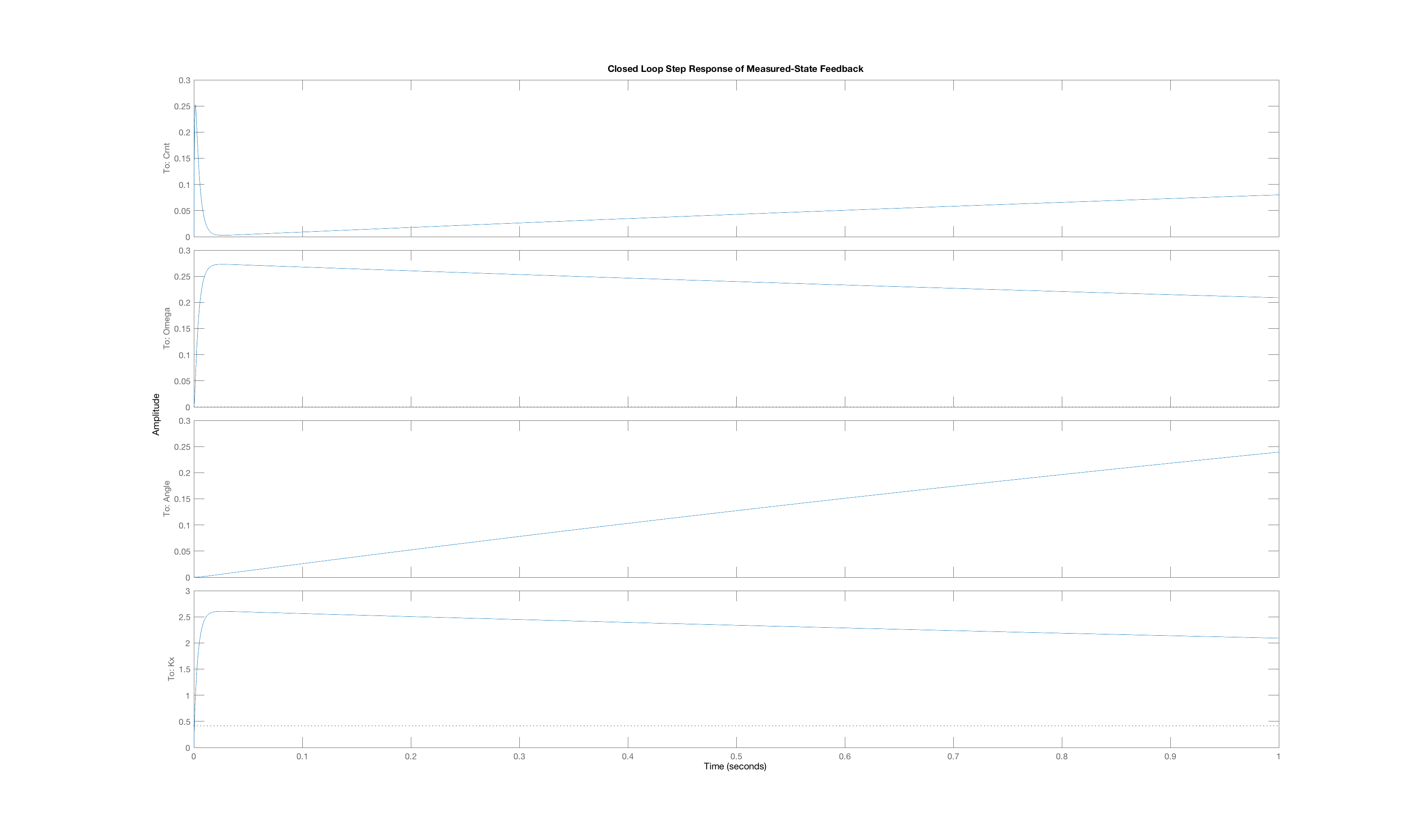
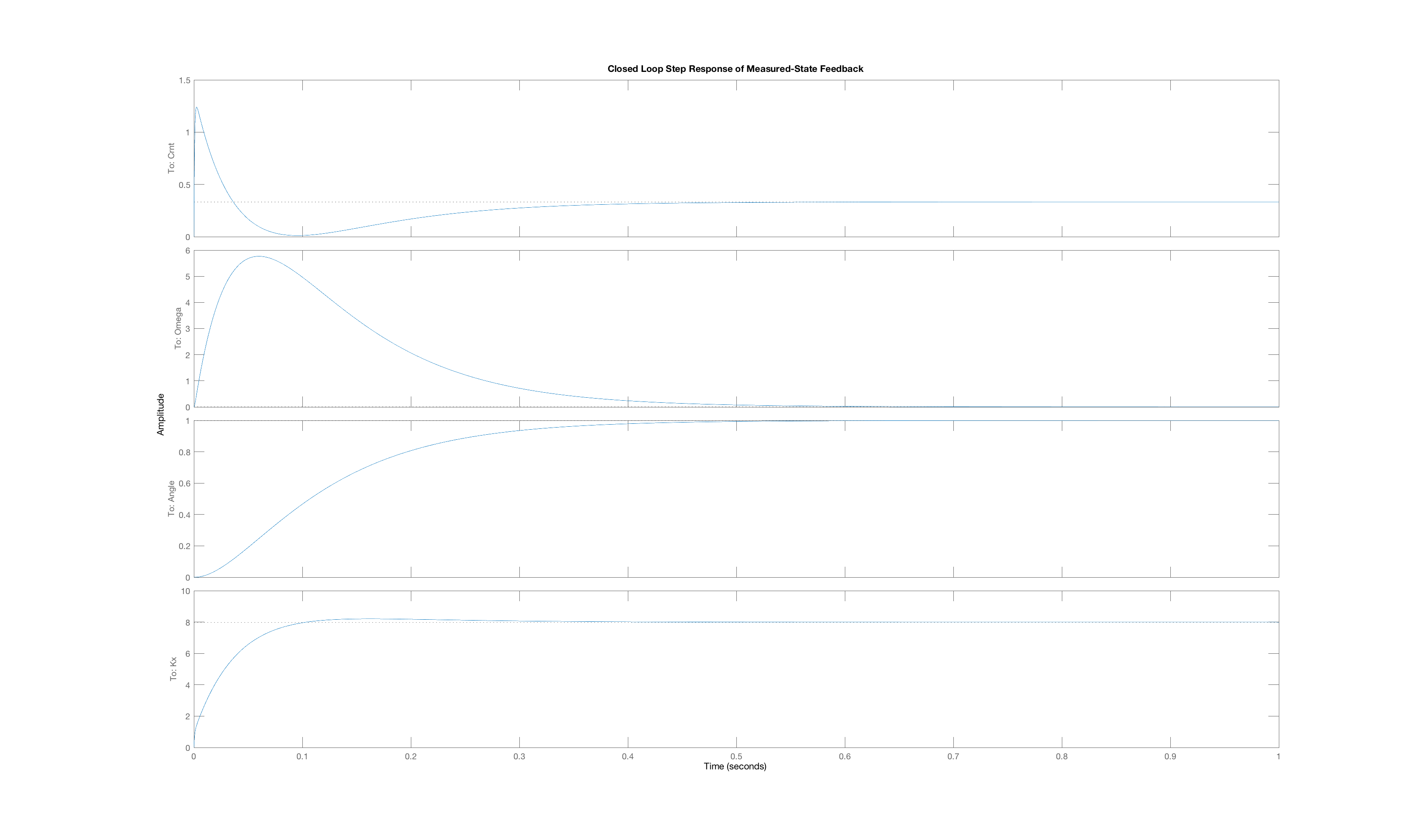
One has to pick ridiculous weights to convince LQR to produces gains that lead to state-feedback systems with highly imaginary poles, but for the Lmotor-driven arm with rubber bands, we did succeed. We used diagonal state weighting, and set two of the weights to 1.0, and the third to 10^p, where p is an integer larger than 2 (you will have figure out what p is, and which state was given a high weight). We then generated a feedback system using the generated gains, and examined the poles. One pole was real and very fast, with a value of -20,000, and the other two poles formed a complex pair, at -1.1 +/- 8.1j. The behavior of this intentionally poorly-designed feedback system is shown below, where the oscillations are very clear.

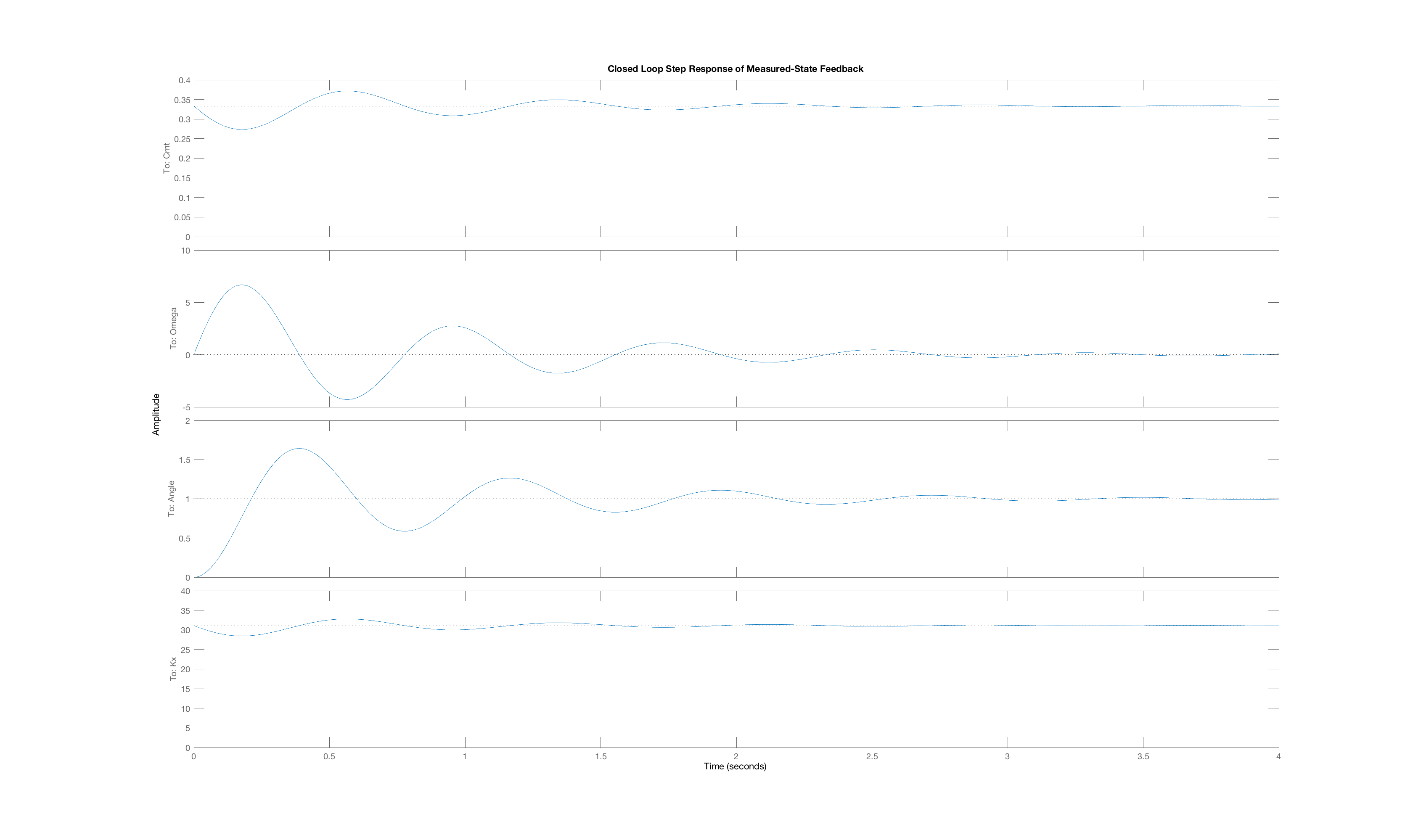
What LQR weights produced the gains used in our oscillatory

Which state was given a high LQR weight?

motor current

Omega

Theta

Loading...

We set the one large weights to 10^p for some integer p, what is p?

Loading...

For this section, use K_b = -0.1.

We computed the poles for the Lmotor-driven-arm plant, that is, the open-loop transfer function from motor-voltage input to arm-angle output. We also noticed that one pole is much larger than the rest, and its associated \beta in the partial fraction expansion of H(s) was much smaller.

If we prevent the arm from moving, so that \omega = 0 and therefore v_{emf} = K_e \omega = 0, then the transfer function from the motor voltage to the motor current is

Given the non-spinning motor assumption, and using the values above for the Lmotor, what is the numerical value of the pole of the transfer function from motor voltage to motor current (remember the pole will be negative).

Note that one of the open-loop plant poles is very close to the of the motor voltage to motor current transfer function, and both are much larger than other poles in the system.

If we want to avoid the complications of measuring motor current, the particulars of this example suggests an approach. Note that one of the poles of the plant transfer function is very close to the pole of the motor-voltage to motor-current transfer function. And since that pole is real and nearly 250 times more negative than the other two poles of the system, the motor current reacts to changes in the motor voltage more than 250 times faster than the rest of the system. That suggests we use an approximation similar to one we used the propeller arm. That is, let us assume

From the matrix algebra perspective, we are reducing our three-state state-space model to a two-state model by setting

The following snippet of matlab code will eliminate the first variable of a state-space description, assuming that the first row and first column of \textbf{E} are zero. It is incomplete however, you will have to determine the multiplier mul.

% Eliminate the first variable from A and B
pivot = % fill this in!!!
for i = 2:size(A,1)  % Zeros out first column of A and B.
    mul = A(i,1)/pivot; 
    A(i,:) = A(i,:) - mul*A(1,:); % Subtract scaled first row from ith row.
    B(i) = B(i) - mul*B(1);   
end
C = C - (C(1)/pivot)*A(1,:);

% Copy over into reduced size matrices
Er = E(2:end,2:end);
Ar = A(2:end,2:end);
Br = B(2:end);
Cr = C(2:end);

What element of \textbf{A} is the pivot? Please enter your answer in python format. So if your answer is i=2 and j=3, enter [2,3].

What are \textbf{A_r} and \textbf{B_r} for the 2 \times 2 reduced system, and what are the two poles (use K_b = -0.1)?

Now lets compare two approaches for computing state-feedback gains for the Lmotor-driven arm system

1. Use LQR with $\textbf{E},$ $\textbf{A},$ and $\textbf{B},$ the matrices for the $3$-state model, to compute the vector of three state weights, $\textbf{K}$.
2. Use LQR with $\textbf{Er},$ $\textbf{Ar},$ and $\textbf{Br},$ the matrices for the $2$-state reduced model, compute the vector of two reduced state weights, $\textbf{K}_{reduced}$. Then prepend the vector with zero, to get a vector of three state weights, $\tilde{K} = [0, K_{reduced}]$.

Suppose we use LQR with input weight R = 1.0 and diagonal state weights Q as [0,1,5000] (or just [1,5000] for the two-state system). What are the LQR gains for the three-state and two-state models of the Lmotor-driven arm.

What were the three feedback gains for three-state model (enter as a python list, e.g. [3,7,12])

Loading...

What were the two feedback gains for two-state model (enter as a python list, e.g. [3,7])

Loading...

As you probably noticed, eliminating the state associated with the motor current did not significantly effect the step response, and you probably also noticed that the gain on the motor current state was quite small. Suppose instead we use a different motor, one with four times the inductance, so that L_m = 0.02, and one forth of the series resistance, R_m = 1.75. What are the poles of the three-state model and what are the poles of the two-state model(derived from assuming L_m\frac{di_m(t)}{dt} \approx 0) for this new system?

poles of the open-loop three-state system

Loading...

poles of the open-loop reduced (two-state) system

Loading...

Suppose we use LQR with input weight R = 1.0 and diagonal state weights Q as [0,1,5000] (or just [1,5000] for the two-state system). What are the LQR gains for the three-state and two-state models of the new-motor-driven arm.

What were the three feedback gains for three-state model (enter as a python list, e.g. [3,7,12])

Loading...

What were the two feedback gains for two-state model (enter as a python list, e.g. [3,7,12])

Loading...

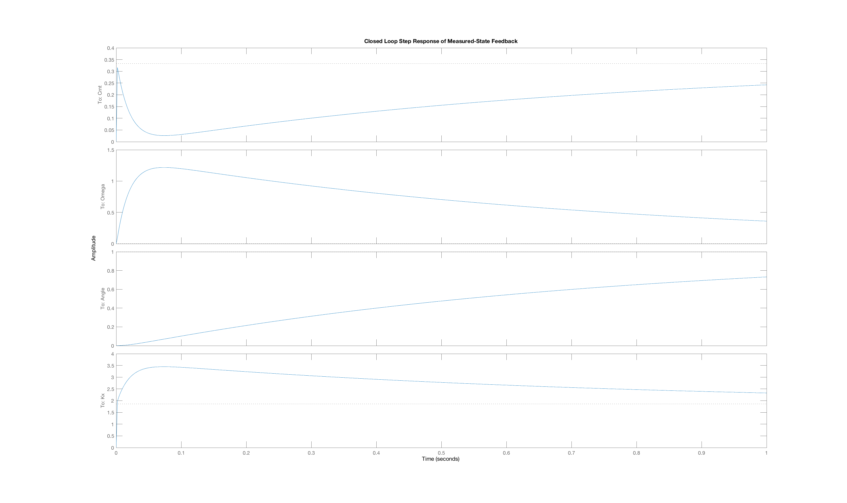
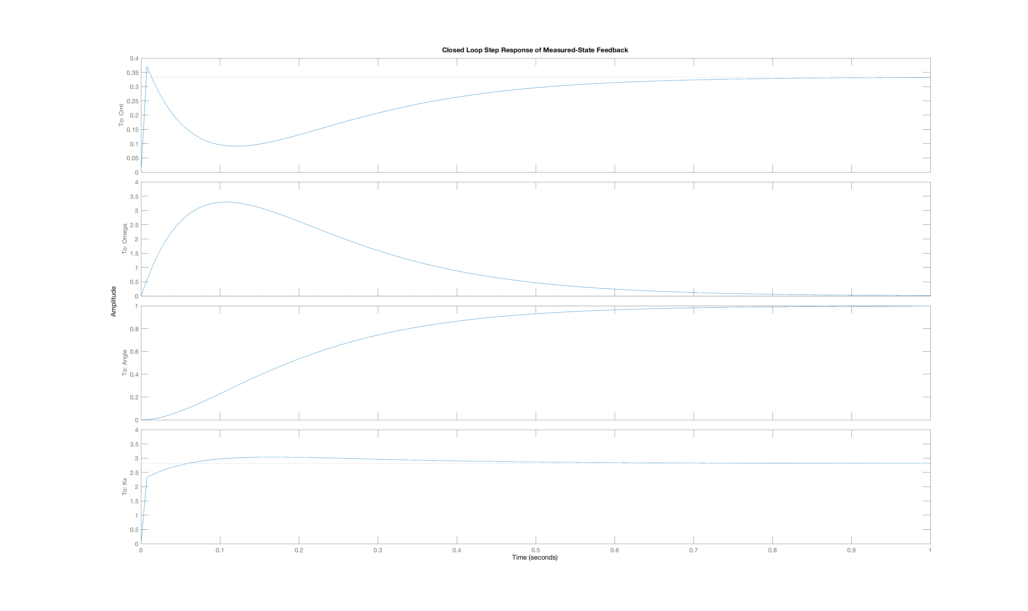
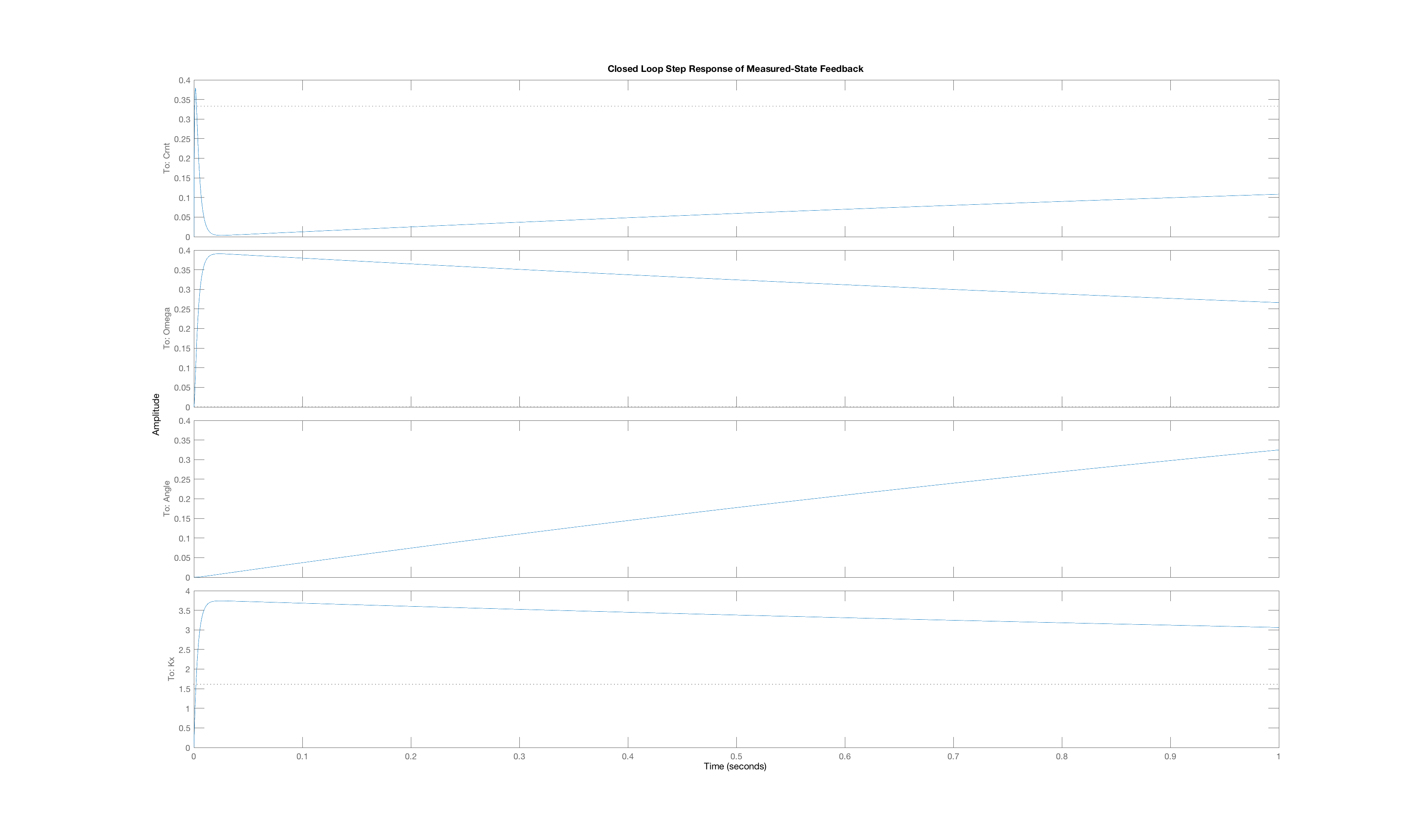
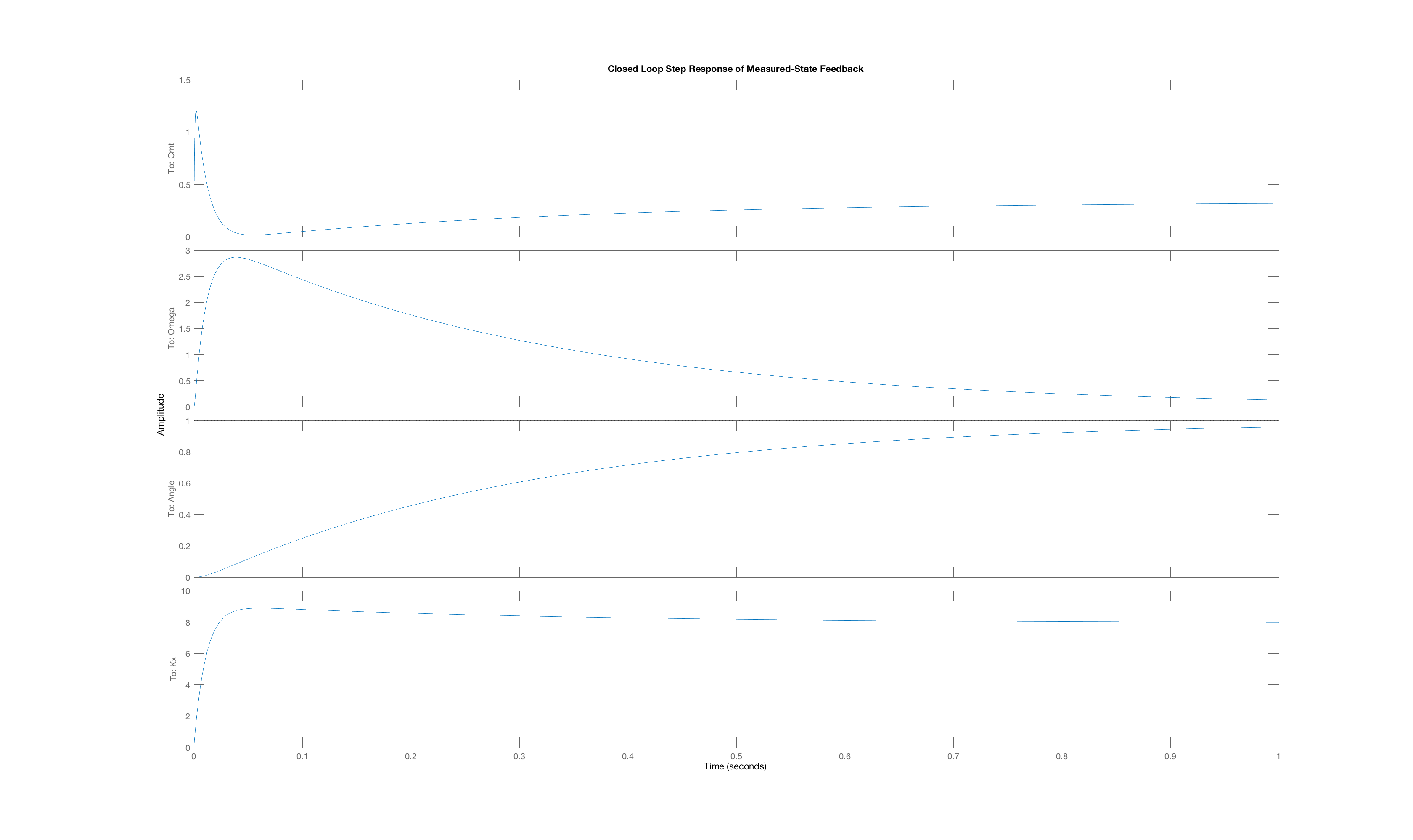
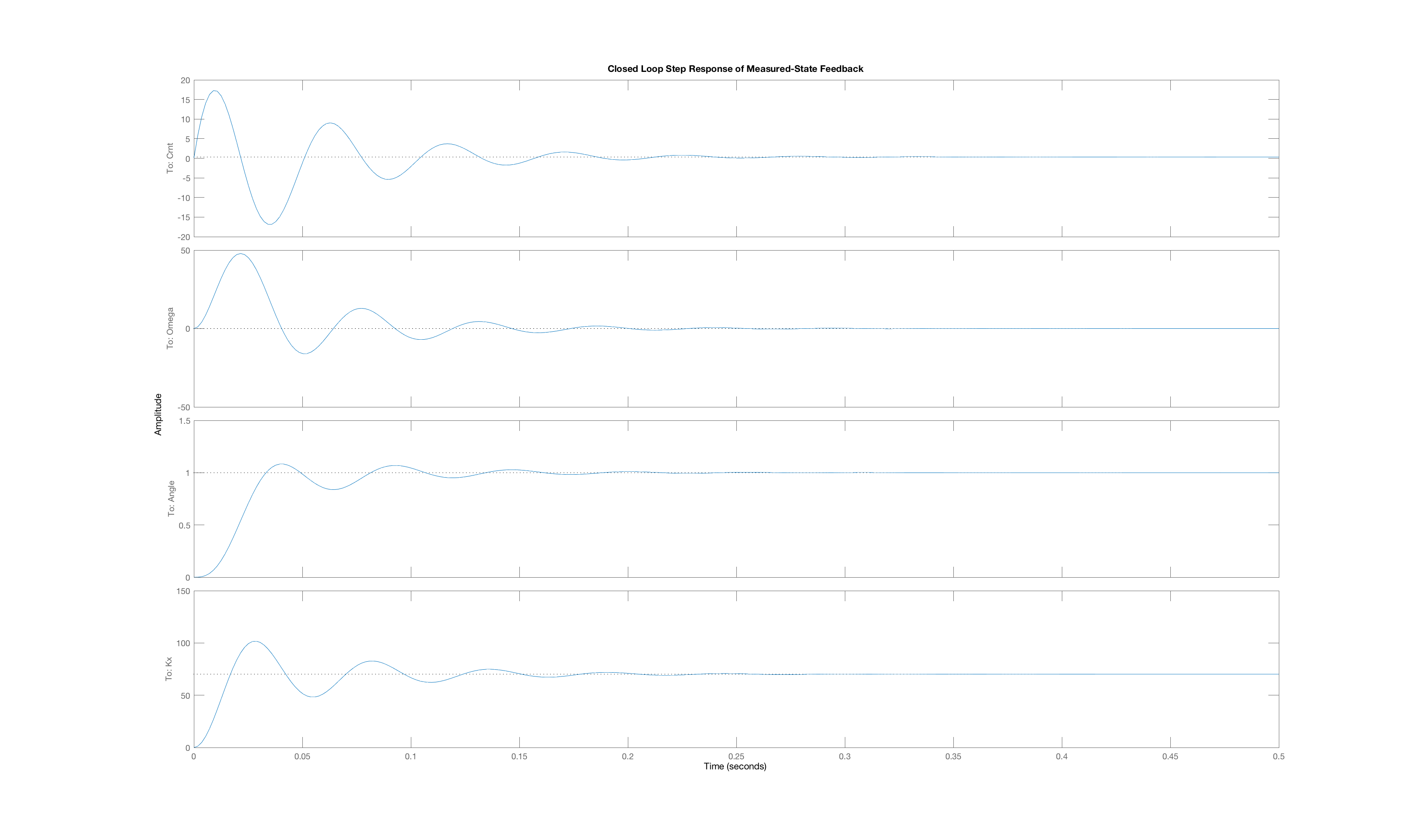
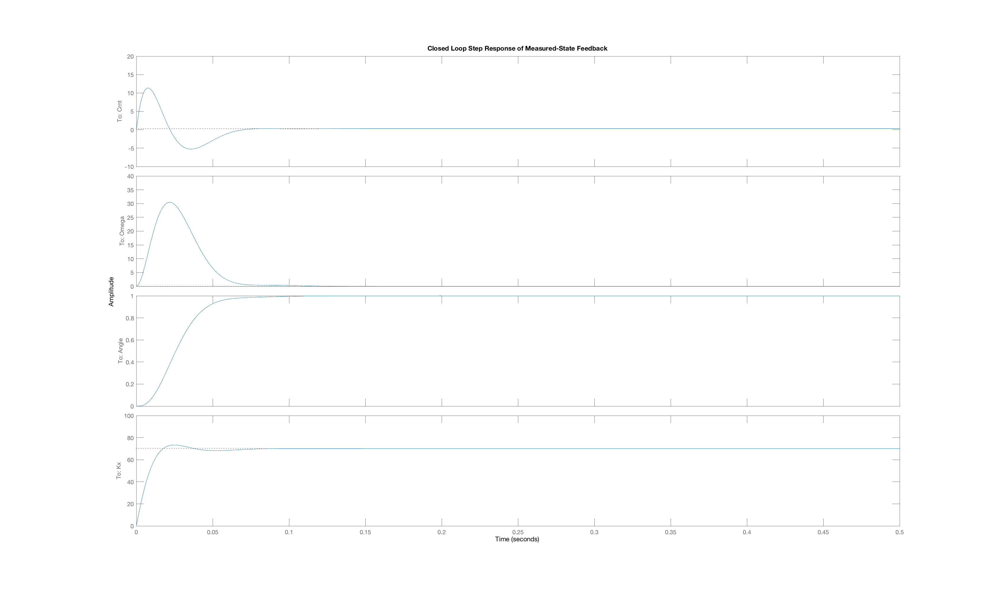
Below we have plotted three closed-loop step responses generated by three of the four senarios above:

1. The Lmotor-driven arm using feedback gains computed with the three-state model,

2. The Lmotor-driven arm using feedback gains computed with the reduced two-state model,

3. The new-motor-driven arm using feedback gains computed with the three-state model,

4. The new-motor-driven arm using feedback gains computed with the two-state model.

Case A

Case B

Case C

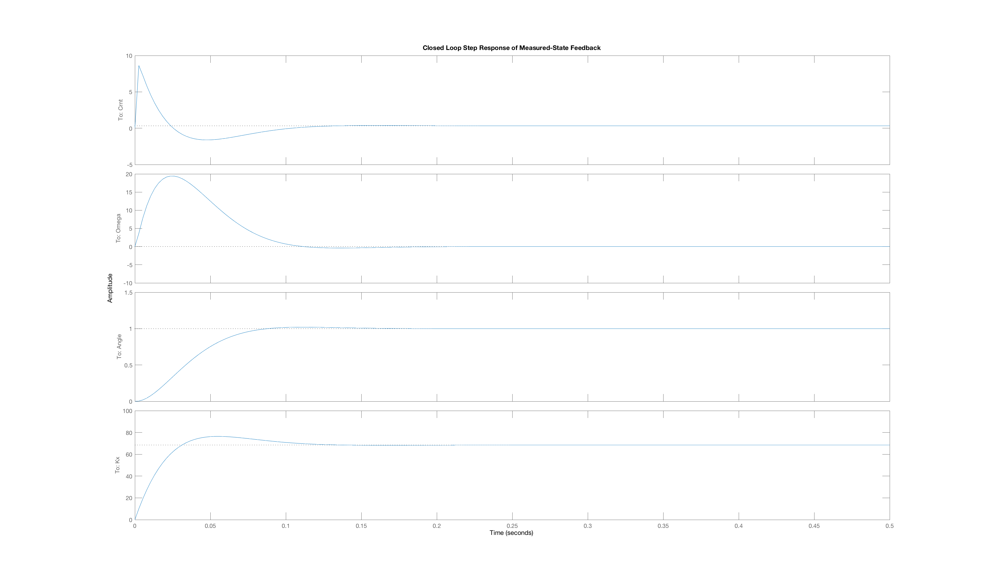
Order the plots using their letters so that the plot order matches the order of the four senarios above. That is, if you fill in the answer

ABCC

then you mean that plot A is the best match to the closed-loop step response senario (1) above, plot B is the best match for the closed-loop step response for senario (2), etc. Obviously, you will need to use one plot twice.

Plot Order =

Loading...