Proportional Control and Difference Equations
Please Log In for full access to the web site.
Note that this link will take you to an external site (https://shimmer.mit.edu) to authenticate, and then you will be redirected back to this page.
A robot that measures obstacle distances ten times a second is placed five meters from a wall. The robot is programmed to move with a velocity negatively proportional to the distance from the wall. We set the velocity negatively proportional to distance to the wall because a robot moving with a positive velocity is moving away from the wall. As the robot gets closer to the wall, it should slow down, but what really happens?
To model how the robot moves towards the wall, we start by representing its distance measurements as a sequence, d, where d[n] is the n^{th} measured distance and d[0] = 5. The difference between d[n] and d[n-1] can be related to the robot's velocity and the time between measurements,
Since the robot's velocity was programmed to be negatively proportional to its distance to the wall,
If we do not want the robot to crash into the wall, or equivalently, if we do not want d[n] to become negative, we now know that the first-order LDE's natural frequency must be non-negative. In addition, if we want d[n] to decay to zero (so that we end up next to the wall), the natural frequency must be less than one. Ensuring that 0 \le \lambda \lt 1, or equivalently, that 0 \le \left( 1 - 0.1 K_p \right) \lt 1, yields constraints on K_p as in
Consider the following questions carefully before moving on to the next section:
- What happens if K_p is very near but \gt 0?
- What happens if K_p is exactly 10?
- What happens if K_p is 11?
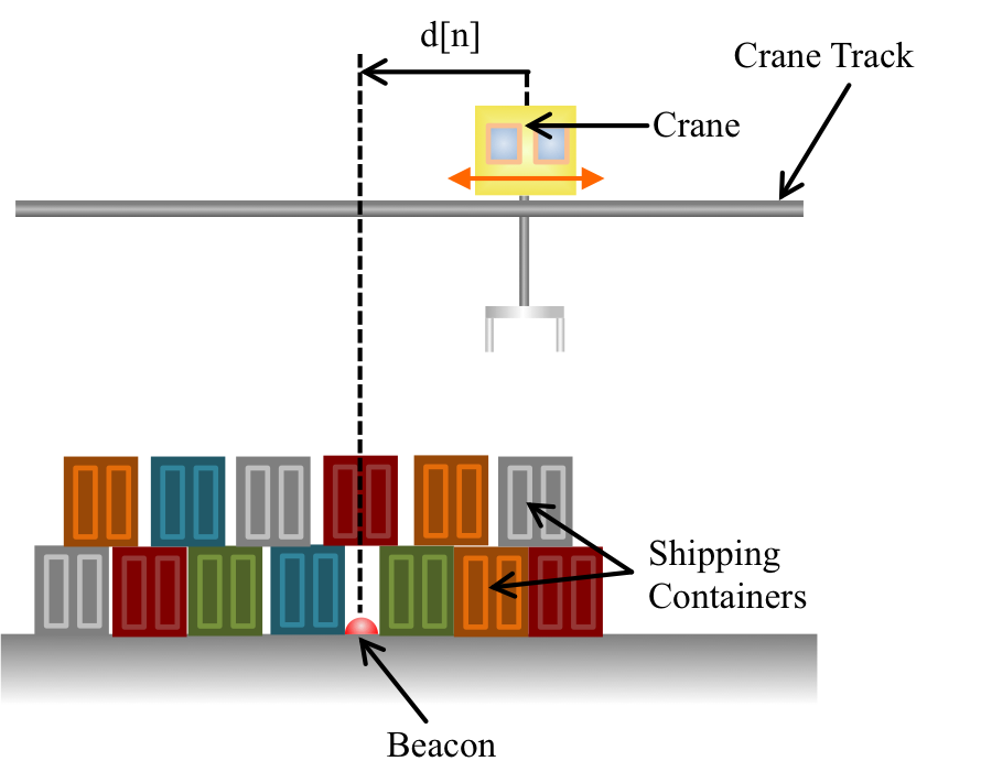
Let us return to the cargo crane traveling on track above a buried beacon, as shown in Figure 1. The crane measures its signed distance to a beacon every \Delta T seconds, where by signed distance, we mean that the distance is negative if the crane has not yet reached the beacon (left of the beacon in Figure), and postive if the crane has traveled past it (right of beacon in Figure ). The crane is intended to self-drive. That is, it can reposition itself on the track automatically, in response to a desired position request.
We are going to assume that the crane has an internal feedback controller that adjusts acceleration to achieve our requested velocity, and that we must design an external position controller.
To model how the crane moves along its track, we will represent the crane's measured distance to the beacon as a sequence, d, and its controlled velocity as a sequence v, where d[n] and v[n] are the n^{th} measured distance and controlled velocity respectively. We can relate the measured distance, d, to its velocity, v, as
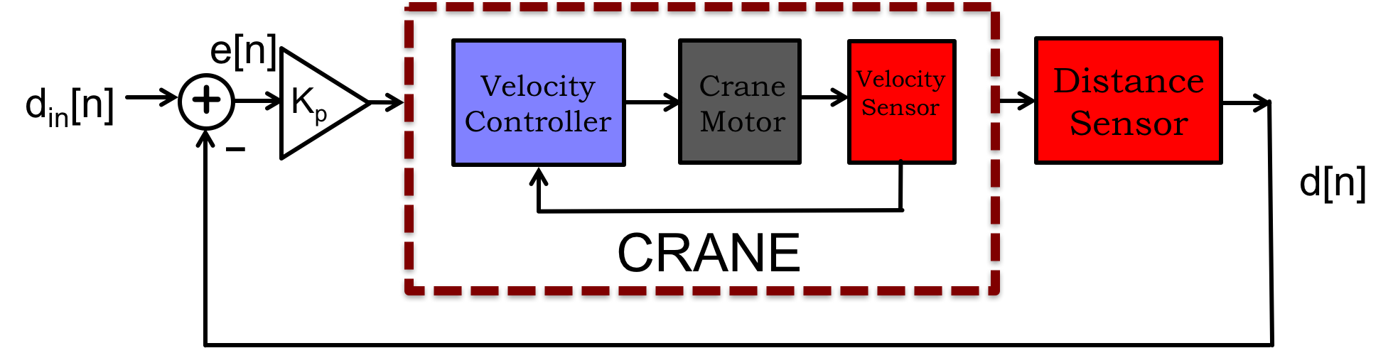
We denote desired position along the track, also the input to our position controller, as the sequence d_{in}, and a proportional feedback approach to controlling the crane would be to make the crane velocity proportional to the difference between the desired and measured crane positions, as diagrammed in the Figure above. Then the velocity is given by
where K_p is the proportional gain and d_{in} is the input, or desired, position.
In order to determine the performance of this proportional-feedback approach as a function of gain, we substitute the control formula in to the distance-velocity relation for the crane,
We know how to solve homogenous LDEs, but we now need to learn about including inputs.
For any system we are trying to control, we will presumably try to influence its outputs by changing its inputs, so we will need to add an input to the homogenous LDE models we already know. In the first-order case, the general form of an LDE with an input is
A delayed unit sample with delay n_0 is given by
As a formal matter, systems described by LDEs are completely characterized by the output due to a unit sample input, referred to as the unit sample response, but that is a digression for us. Formality aside, we can reason about systems by examining their response to a unit sample.
If y[0] = 0, and the input is a delayed unit sample, x[n] = \delta[n-n_0], then y[n] has a familiar power series form that can be derived in a few steps.
For n \le n_0, y[n] = 0, and for n = n_0+1,
For n > n_0+1, x[n] =0 and therefore y[n] = \lambda y[n-1], the generating difference equation for the power series. Iterating yields
In the stable case, that is if |\lambda| \lt 1 ,
A delayed unit step with delay n_0 is given by
for which we use the compact notation x[n] = u[n-n_0]
Given a unit step input, x[n] = u[n-n_0], and y[0] is still zero, then y[n] = 0 \;\; n \le n_0 and y[n_0 + 1] must equal b \; x[n_0] = b \; u[n_0-n_0] = b \;. For n > n_0+1, x[n] =1 and therefore
If we write out the terms, we can see the pattern,
Iterating yields a representation of y as a power series sum,
In the stable case, that is |\lambda| < 1 ,
which can be seen by summing the series.
For the stable case, |\lambda| \lt 1, if the input eventually becomes constant, such as in the delayed unit step, we are often only interested in behavior for large n. If so, there is an easier approach to determining y[{\infty}] , a surprisingly useful trick more generally.
Suppose x[n] =1 for n > n_0 and |\lambda| \lt 1. In this stable, constant input, case, y[n] and y[n-1] both approach y[{\infty}] for large n, so
There are many ideas hidden in the above simple formula, and they are best exposed by answering questions. Questions:
- Given b \; > 0 and x[n] = u[n], if \lambda = -1 does y[n] remain bounded?
- For the \lambda = -1 case, does y[{\infty}] exist?
- Does y[n] remain bounded if \lambda = 1?
- Given b \; > 0, and x[n] = u[n], what value of \lambda minimizes y[\infty] when it exists, and what is that minimum value.
Answers:
- Yes, y[n] is bounded.
- No, y[{\infty}] does not exist as y[n] alternates between 0 and b \; forever.
- If \lambda = 1, y[n] is unbounded, and y[{\infty}] does not exist.
- Setting \lambda very close to -1 minimizes y[\infty], which is bounded from below by \frac{b \;}{2}. But then y[n] oscillates and decays very slowly.
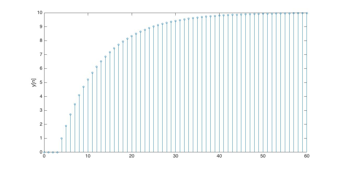
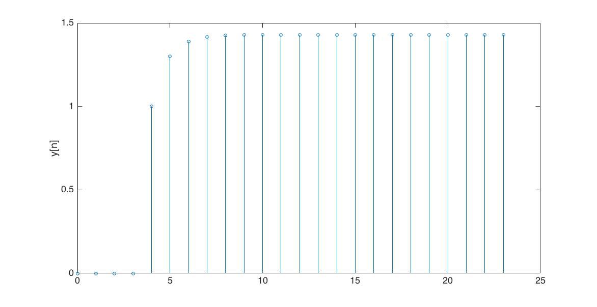
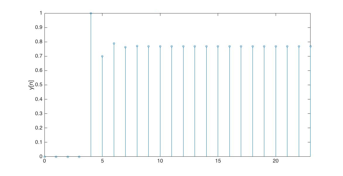
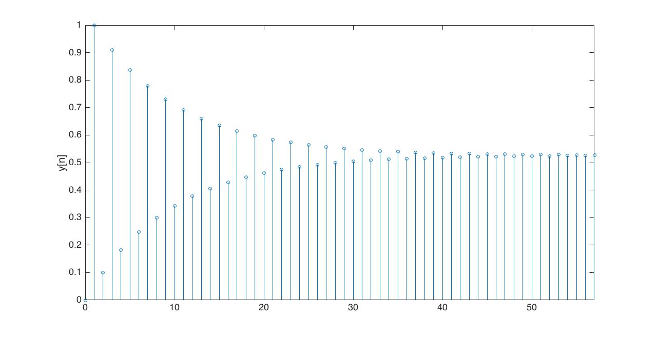
And one last use of y[{\infty}], we use it to construct the entire step response. If y[0] = 0, x[n] = u[n-n_0], and |\lambda| \lt 1, then y[n] = 0 for n \le n_0 and
In the Figures below we show the behavior of the step response for several different values for \lambda. Notice the large n values in the plots. For example, even if \lambda \lt 0, the large n value is still positive.
For the following problems,
A: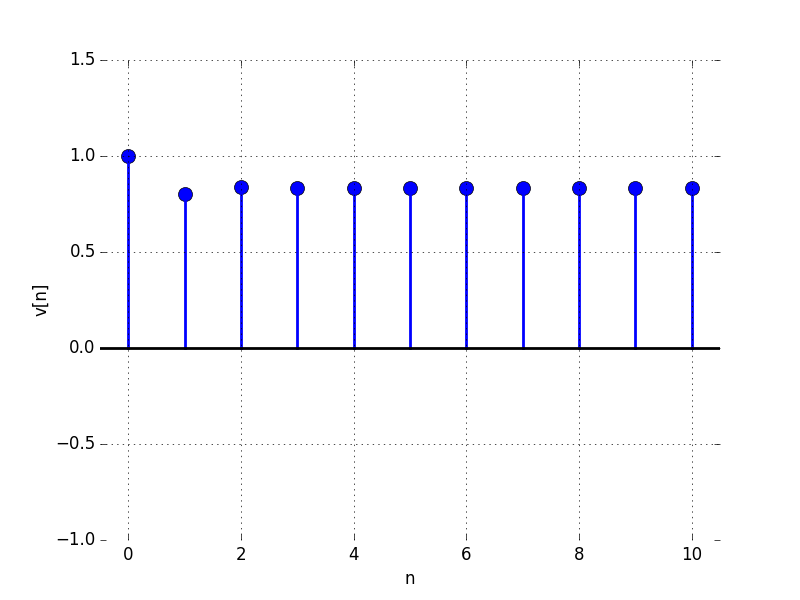
|
B: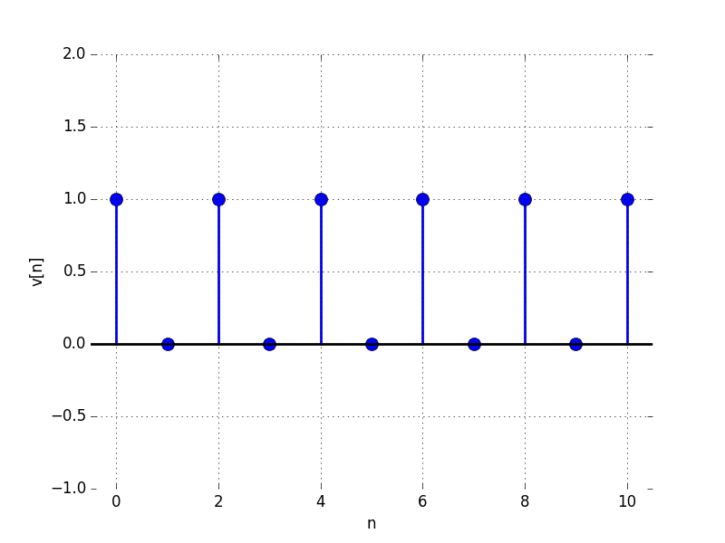
|
C: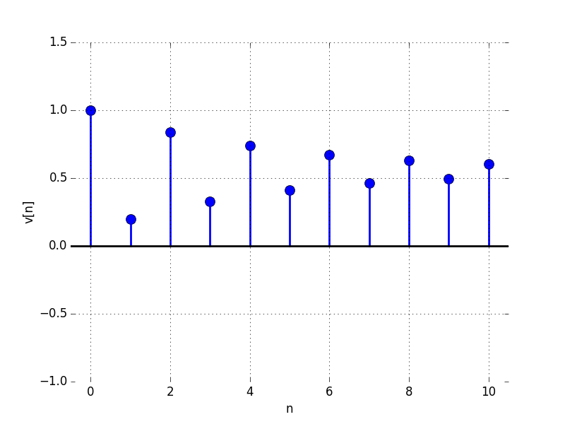
|
D: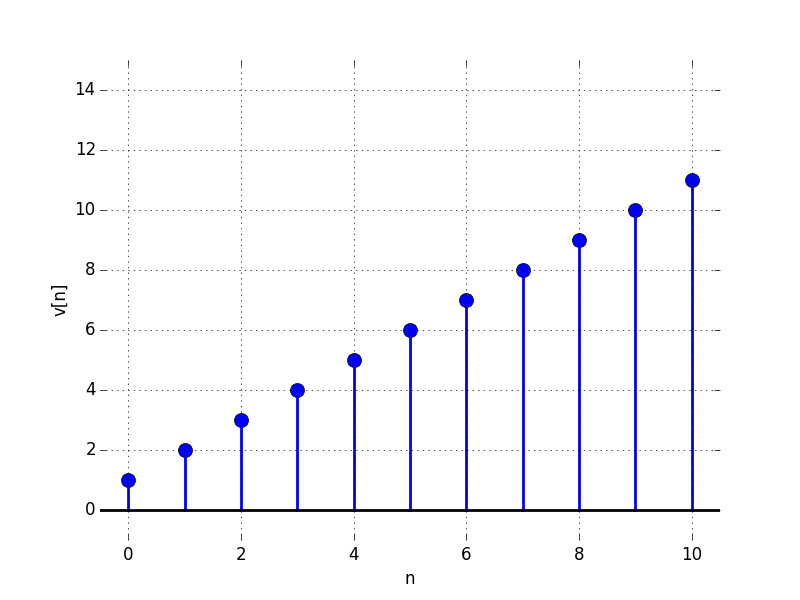
|
E: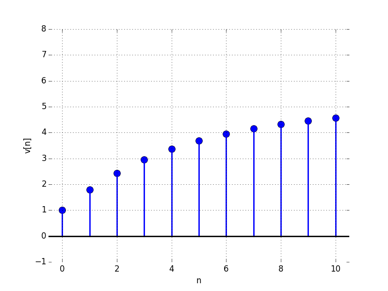
|
F: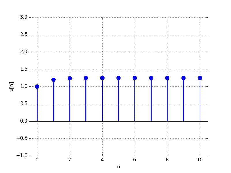
|

For what value of \lambda is the limit as n \to \infty of v[n] equal to:
A model for a proportional feedback system is given by the difference equation
A: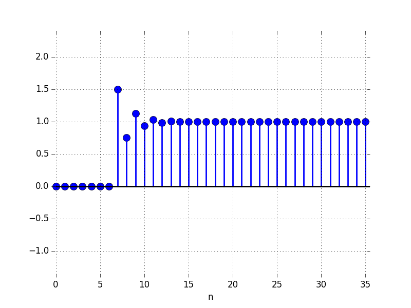
|
B: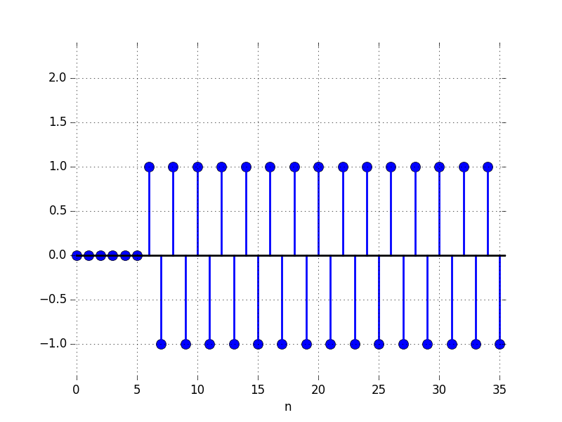
|
C: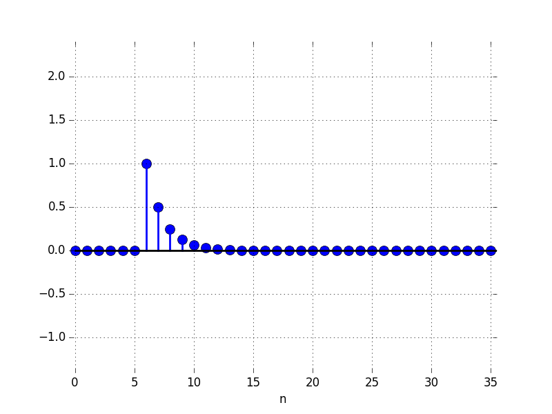
|
D: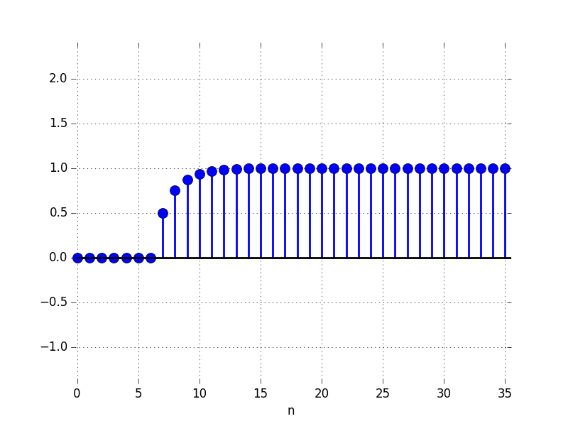
|
E: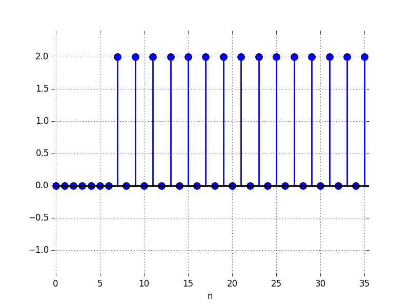
|
F: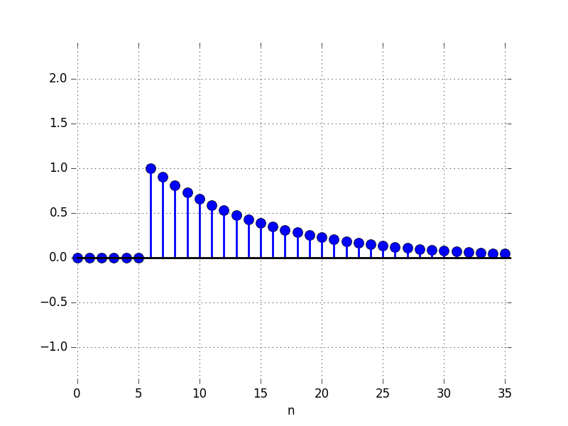
|
G: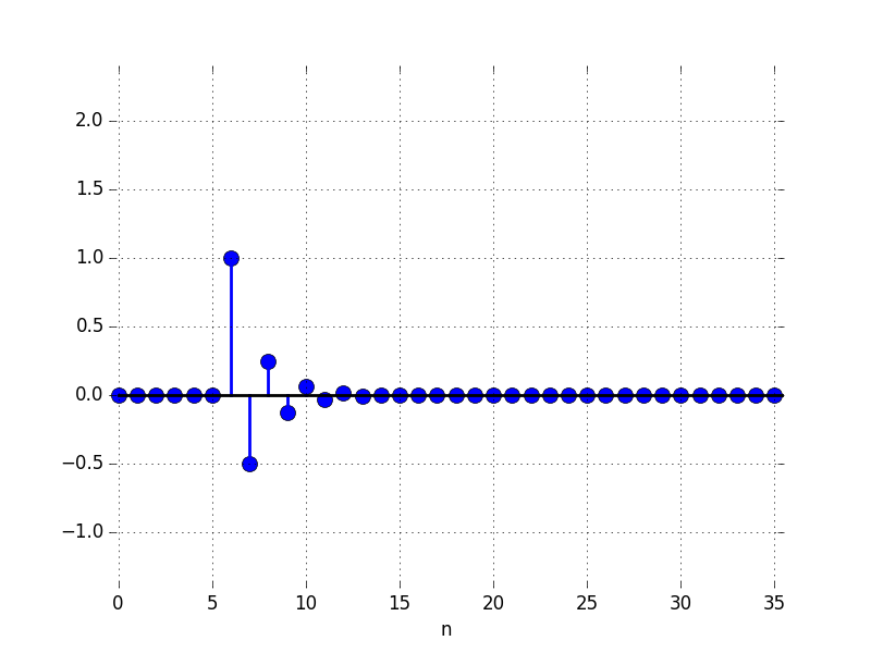
|
H:
|