A Disturbance in the Force

Quick Reference

NOTE

When the new sketch (6310_PROP_24_SWEEP) is uploaded to the Teensy, it sets K_p, K_d, and K_i to 0.
To get non-zero values, you must set them via the serial plotter send window.

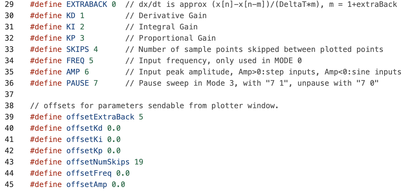
Serial Plotter Send Window Indices and offsets

Links

• Build instructions for adding second motor are at the end of section three in here.
• Sketch for this lab is here.
• Matlab script for week B is here.

Task Summary

Week A

1. Add second motor to your arm, download the new sketch, recalibrate angle sensor offset, and level the arm. (Checkoff 1).
2. Set K_i = 4.0, K_p = 0.5, and find the smallest value of K_d for which the system is stable (step response settles to its steady-state in less than 5 seconds).
3. Measure the frequency of the oscillation in the step response, and the magnitude and phase of sinusoidal steady-state responses for several input frequencies.
4. Disturb the arm by fanning it, and find the "fanning resonance frequency" that maximizes the disturbance response.
5. Consider how the following are related:
   • the frequency of the oscillations in the step response,
   • the frequency that maximizes the sinusoidal steady state response
   • and the frequency that maximizes the disturbance response (Checkoff 2).
6. Repeat 2->6 with K_i=0, K_p = 2, and for this case find a new smallest K_d for which the step response settles in less than five seconds(Checkoff 3).

Week B

Adjust \gamma_a and \beta in the provided matlab model so that the input-output frequency response of the model matches the steady-state magnitude and phase of your arm's input-output response at a few points.

Derive the disturbance to output transfer function, and update the matlab script so that it also computes the disturbance frequency response. Fan your arm to demonstrate that your model's disturbance frequency response accurately predicts the most disturbing frequency.

Use your model (and matlab) to design a controller with better disturbance rejection by examining the disturbance frequency response. Fan the arm to demonstrate the improved disturbance rejection of your better controller.

Double the Fun

Add a second motor: clip it into the counter-weight on the right side of the arm (see the end of section three in the assembly guide). Slide the position of the second motor on the arm so that the arm is balanced (stays level when the power is off). Connect both power supplies to the controller board and connect your laptop to the Teensy. Download the 6310_PROP_24_SWEEP sketch, upload it to the Teensy, and start the serial plotter. Note that the offsets for K_p, K_d, and K_i are zero. You will have to change these values to get enough feedback for the arm to level itself.

Transfer your angle sensor calibration (AngleOffset) BUT NOT THE NOMINAL COMMAND to the new sketch, and verify that the measured \theta_a is zero when you hold the arm level. Once the sensor is calibrated, adjust the black potentiometer (in the upper right hand corner of the board) to balance the right and left propeller forces so that the arm holds itself level.

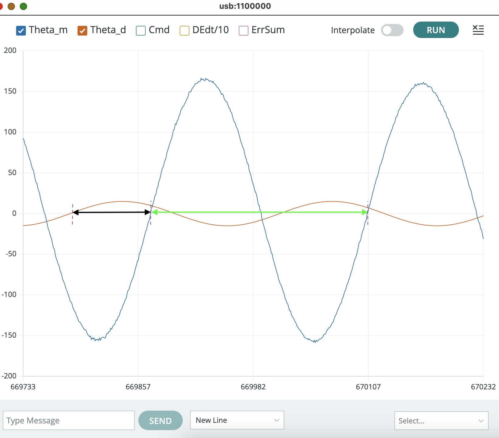
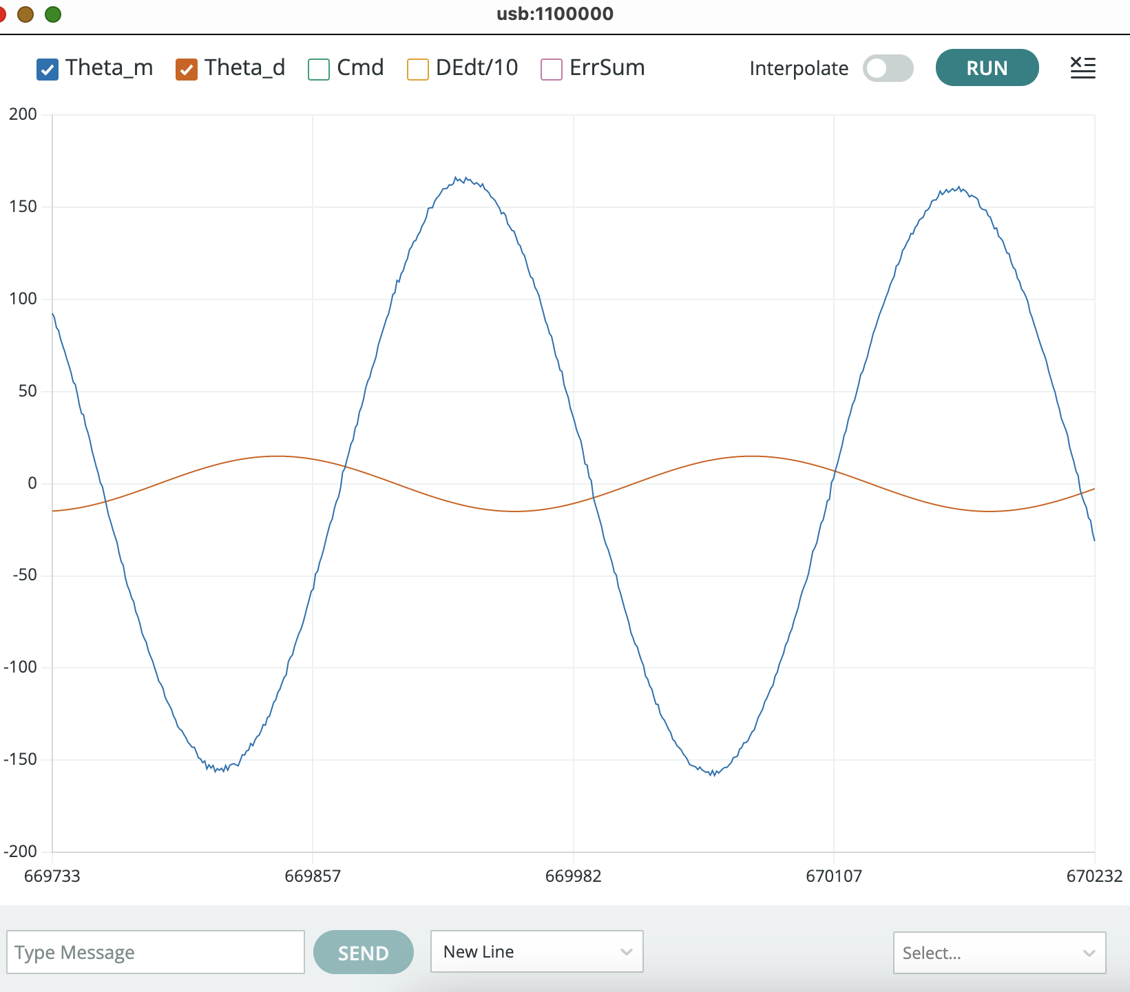
The figure below shows the serial plotter output from running the new sketch with a sinusoidal input (in red) and the resulting measured angle (in blue). Notice the two intervals measured on the plot, one denoted with a black double arrow and the other with a green double arrow. How does the ratio of those two intervals relate to the phase difference between the two plots?

Steps, Sinusoidals and Interference.

Step response.

Set K_p=0.5; K_d=0.2; K_i=4.0 and then type "6 0.1" and "5 0.1" to generate an input that toggles between -0.1 and 0.1 every 5 seconds (two transitions in a ten second period). Then try a few different values for K_d. You should be able to find a K_d between 0.1 and 0.3 that produces a step response similar to the one in the following video.

Notice that the step response plotted in the video above is barely stable, but it is stable! Try using your hand to perturb your arm by about 45 degrees, and then let it go. If your arm persists in oscillating wildly, and does NOT eventually level out, your arm is not stable enough, please increase K_d a little (ten percent) and try again.

Measure Frequency Response

In theory, measuring the frequency response of STABLE linear system is easy:

1. Pick a frequency and apply a sinusoid of that frequency to your system's input.
2. Wait for the system's natural responses to die out (they must die out eventually, since the system is stable). What remains will be sinusoidal at the same frequency as the input.
3. Compare the input sinusoid to the output sinusoid and compute the amplitude ratio and the phase difference.

We can measure the frequency response for our two-propeller arm system using the above approach as long as we are careful about three issues described below.

Monitor Motor Commands

While the two-propeller arm is intended to cancel the gravity-induced nonlinearity of the one-propeller arm, the cancellation is only perfect if the arm is perfectly symmetric (so balance the arm as best you can!). In addition, there is still a "clipping" nonlinearity that arises when the controller-generated motor commands exceed power supply limitations. This nonlinearity can usually be avoided by reducing the magnitude of the sinusoidal input, provided the clipping has been detected.

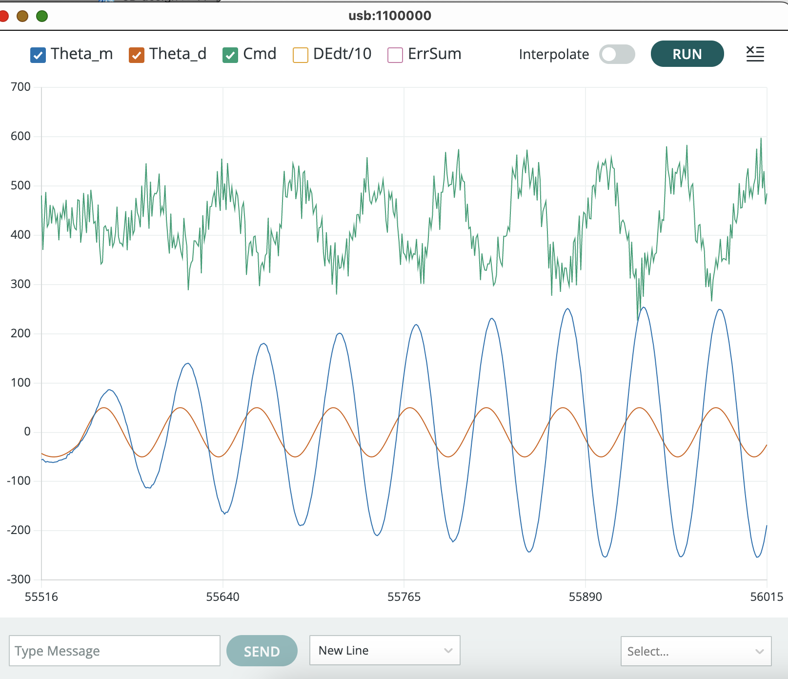
Monitor the motor command plot whenever measuring frequency response, to ensure the commands are not being "clipped" by power supply maximums. The clipping effect is easy to spot, as shown in the figure below. The black arrows point to cases where the motor command (the green curve) flattens, an indication that the controller's commands are being clipped because of power supply limitations.

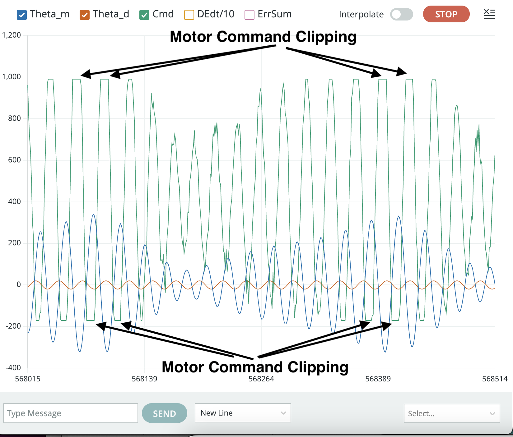
The clipping problem can usually be eliminated by reducing the input amplitude, as shown in the picture below. Avoid reducing the input amplitude too much though, because the microcontroller won't be able to represent the signal accurately. Use index 6 in the plotter window to set a reasonable sinusoidal amplitude (e.g., -0.1).

NOTE: USE NEGATIVE AMPLITUDES, THE SKETCH WILL GENERATE STEPS INSTEAD SINES IF YOU USE POSITIVE AMPLITUDES.

Wait for Steady-State

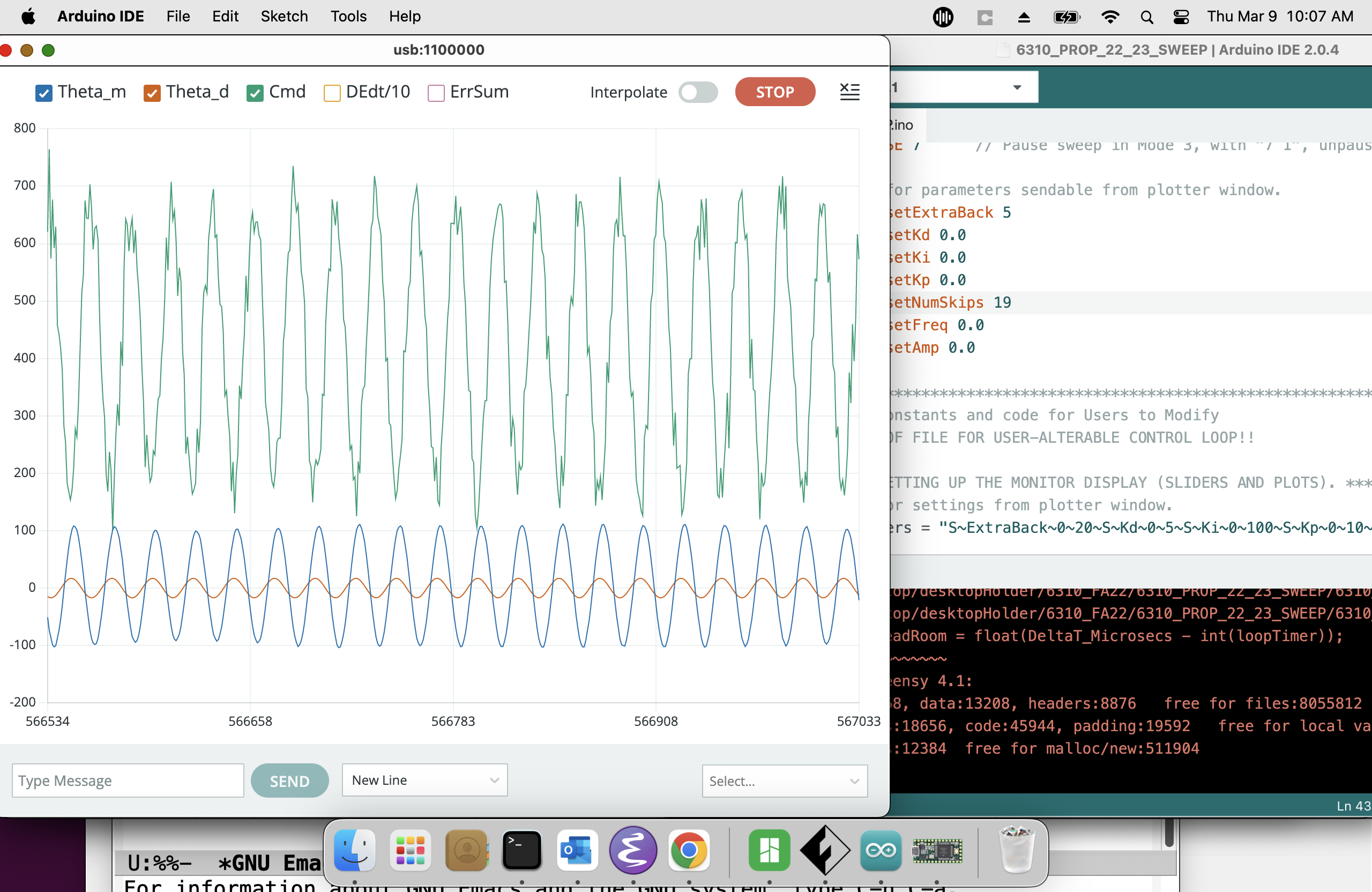
It can take several seconds to achieve sinusoidal steady-state, a typical case is shown in the picture below. Be sure to wait long enough (ten seconds or so) before pausing the plotter and taking measurements.

Spread Samples

In last week’s lab, we sent an update to the serial plotter every 10 milliseconds. For this week, the sketch default is to send an update to the serial plotter every 20 milliseconds. At higher sinusoidal frequencies, it may be helpful to decrease the time between updates and measure time more accurately. The fastest serial plotter update is once per millisecond (zero skips). To set that update rate, type "4 -19" into the plotter send window (as was done to generate the plot below). Note that the default offset for number of skips is set to 19 in the code. As another example, to update the serial plotter every 10 milliseconds, we want to skip 9 samples so type "4 -10"” into the plotter send window.

Checkoff 2

For the second checkoff,

1. Measure the frequency of the oscillation in the step response
2. Measure the amplitude ratio (measured amplitude / input amplitude) and phase shift of sinusoidal steady-state responses for several input frequencies (at least 10 of them). Make plots of amplitude ratio vs. input frequency and phase shift vs. input frequency.
3. Find the the input frequency that maximizes the amplitude of the output, and note the associated output's phase.

Once again, without the integral.

Set K_i=0 and K_p = 2. Then adjust K_d so that you get a "barely stable" step response like in the video below.

Try fanning your updated system, you should be able to excite a resonance, like in the video below. As you can see in the video, at the faster resonance frequency, it can be hard to "match up" to the resonance, please watch until (or skip to) the end to see what that looks like!!

Checkoff 3

For this checkoff,

1. Measure the frequency of the oscillation in the step response, and verify the relation between that frequency and the frequency that maximizes the magnitude of the sinusoidal steady-state response.
2. Try disturbing the arm by fanning it, find the "fanning resonance frequency" that maximizes the response.
3. Note the connection between the frequency of oscillations in the step response, the frequency that maximizes the sinusoidal steady state response, and the fanning frequency that maximizes the disturbance response.

STOP HERE FOR WEEK A!!!!

Continuous Time (CT) Modeling

Last lab we derived an approximate discrete-time (DT) model for the innately continuous-time (CT)propeller arm. We chose discrete-time partly to match our innately discrete-time Teensy-based controller, and partly because discrete-time models, at least the ones formulated as systems of linear difference equations, have explicit solutions in the form of easily computed sums. For this and the next few labs, we will do the reverse. That is, we will derive CT models for innately-CT physical artifacts, and create approximate CT models for our innately-DT controllers.

We are switching to CT because the concepts we are exploring next, transfer functions and frequency response, have a simpler and more intuitive description in CT. And that simplicity will allow us to gain new insights into control system design.

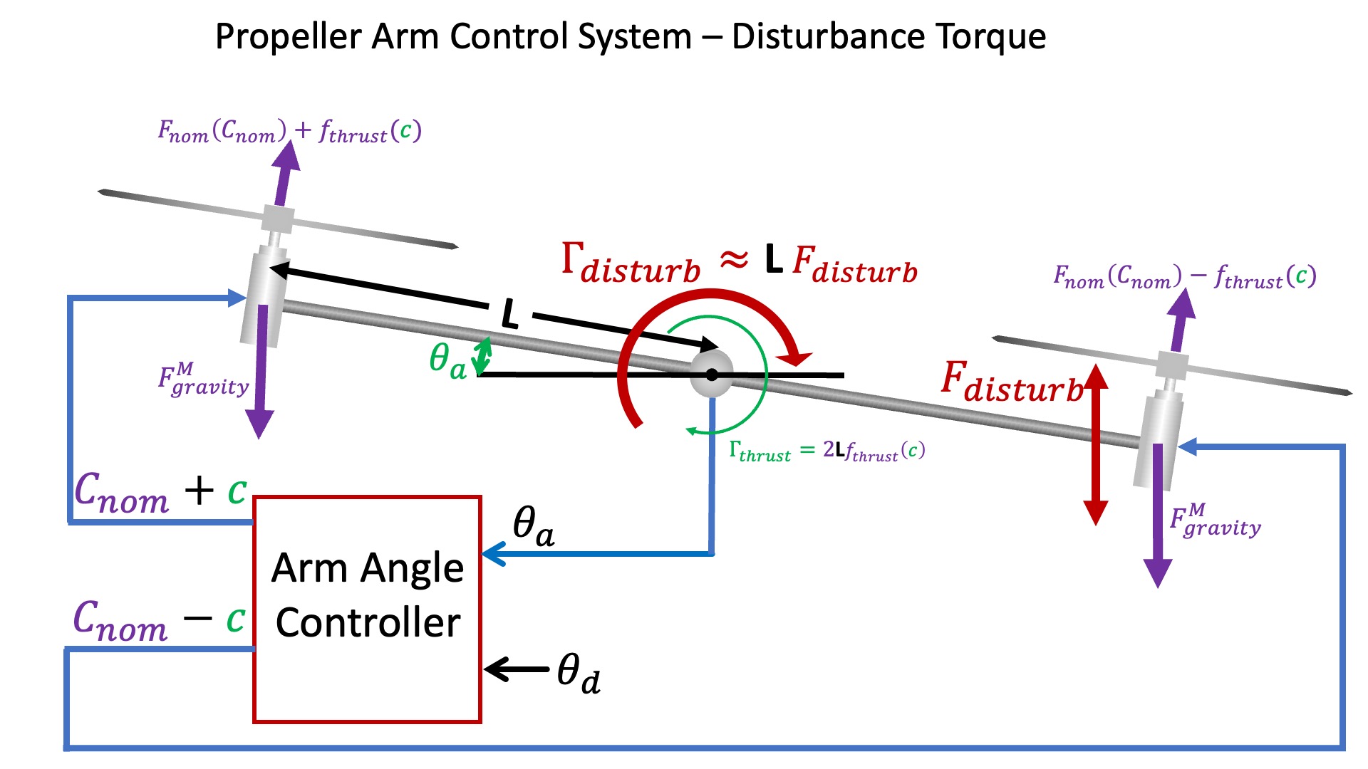
Doubly-Driven Arm

The larger number of forces and torques for the doubly-driven arm are best depicted using a more abstract picture than we used for the singly-driven case, as in the figure below.

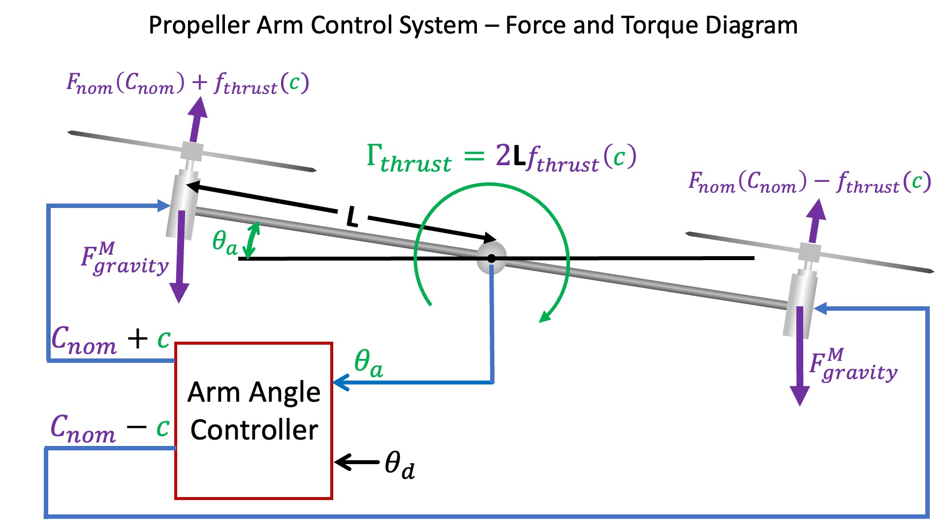
In the above figure, we repeat the definitions of measured and desired arm angles, \theta_a and \theta_d, respectively, show the motor gravity and thrust forces, F_{nom}, f_{thrust}, and F_{gravity}^M, as well as the motor commands, C_{nom} and c. We also explicitly introduce the arm torque, \Gamma_{thrust}, due to the difference in right and left motor thrusts.

In the last lab, we did not model disturbances, and implicitly assumed the net torque on the arm was due to motor thrust alone. Under that assumption, \Gamma_{thrust} was an unnecessary intermediate in the relation between motor command and arm acceleration. This lab is focussed on modeling disturbances, and since our example disturbances (fanning and dropping weights) are torques, their effect on arm acceleration will be easier to model if we can add them to an explicit \Gamma_{thrust}.

Discrete-Time (DT) to Continuous Time (CT)

In the first propeller-arm lab, we related the change in arm angle, \theta_a, to the arm angular velocity, \omega_a,

an approximation to the CT differential equation,

Similarly, we related the change in arm angular velocity to the arm angular acceleration, \alpha_a,

an approximation to the CT differential equation,

Block Diagrams

Simple Model, Simple Control

In our simplest arm model, angular acceleration is assumed proportional to motor command, and in the simplest controller, the motor command is assumed proportional to angle error. In discrete time,

and in continuous time where K_p is the gain of the proportional feedback.

Note that the DT and CT equations are almost identical, the only difference it the replacement of [n] by (t)? Is that generally true?

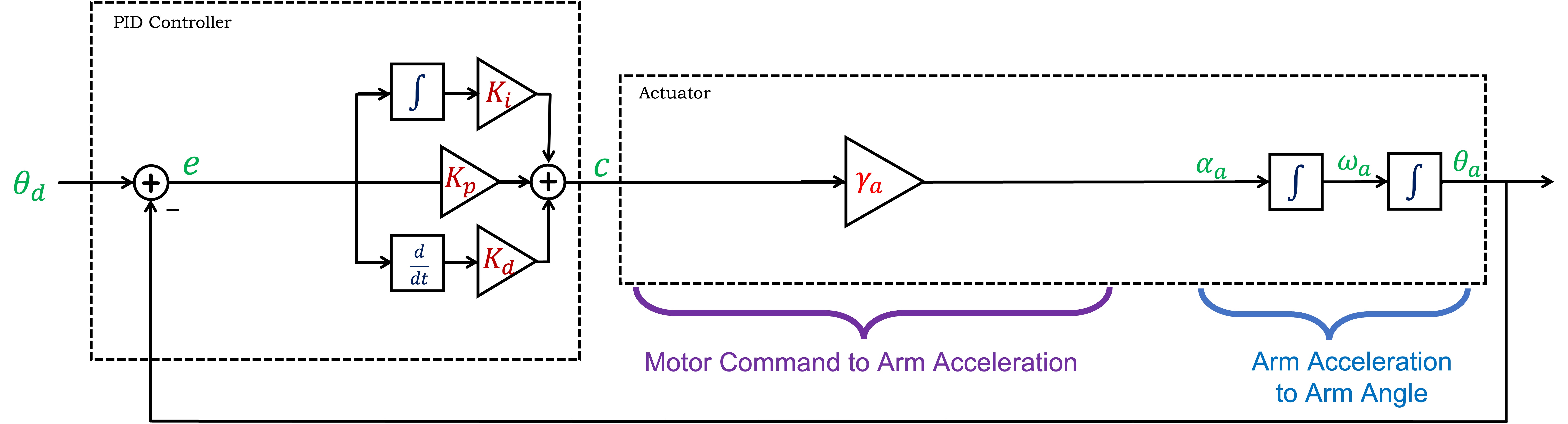
We can combine the equations for the arm, from the previous section, and the equations for the motor and controller, above, into a CT block diagram.

Note that in the CT diagram, we combined blocks with integral operators rather than combining blocks with derivative operators, a choice that parallels our intuition. That is, the system's controller sets the acceleration, which integrates to velocity, which in turn integrates to position, which we then measure and feed back.

Simple Model, PID control

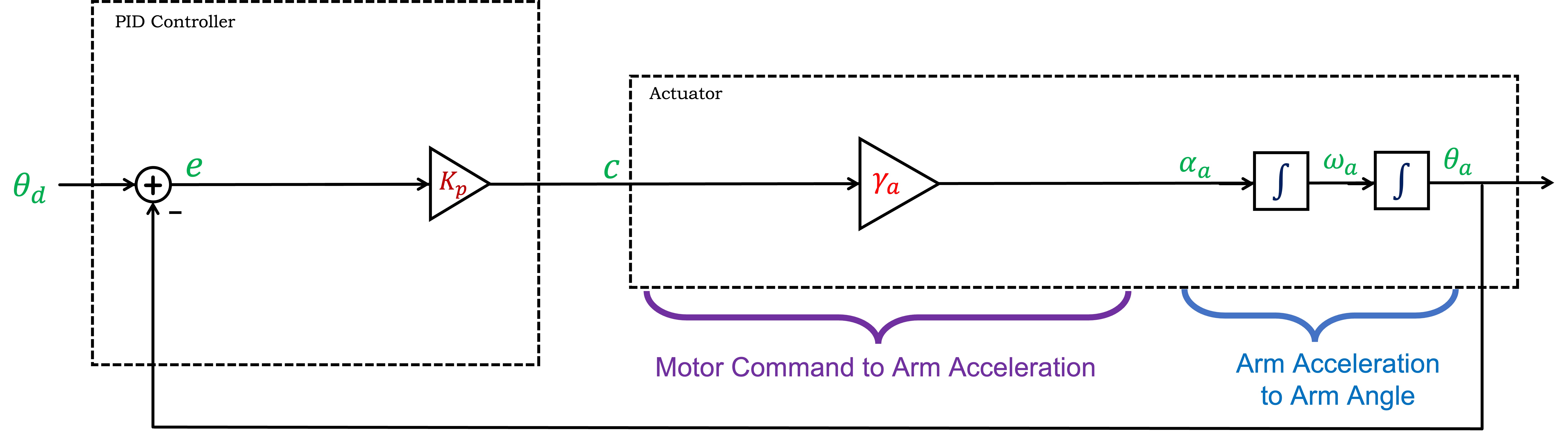
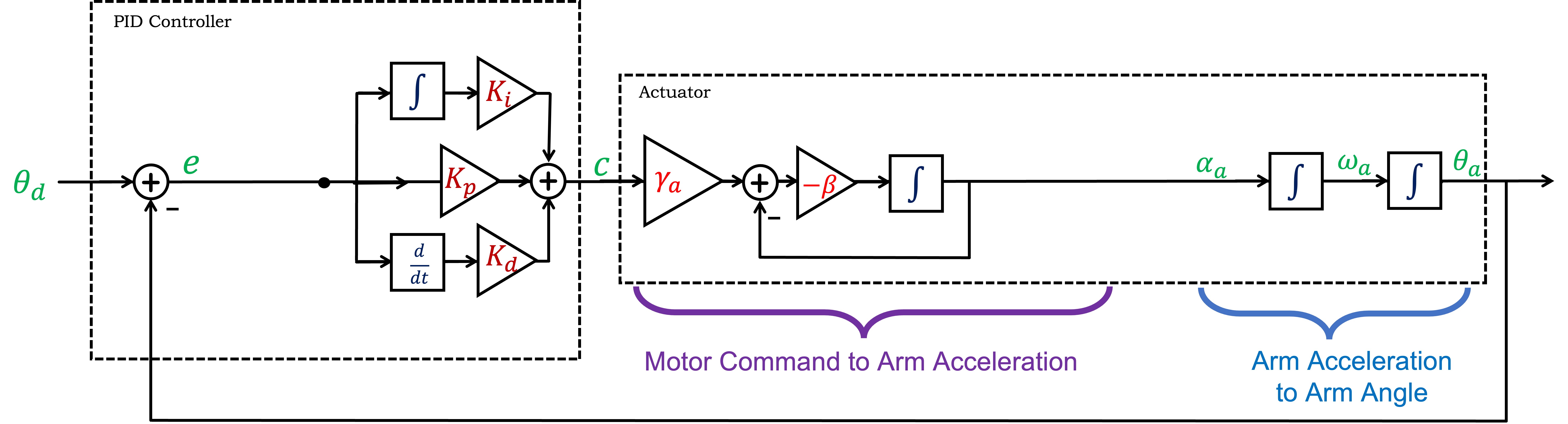
We know that proportional feedback alone can not stabilize the propeller arm, so derivative feedback is essential, and we also know that integral feedback improves steady-state tracking. Including all three (P,I,D) in a CT block diagram is easy, because the integral and derivative blocks can be used directly, as shown below.

Note that even though we are representing the arm control system with a CT block diagram, the derivative and integral controller terms will still be approximated on the microcontroller using scaled angle error differences and running sums. Nevertheless, we will continue to approximate the DT behavior with a CT representation, because we can model the system with simple block diagrams and develop intuition and insight.

Non-instant Motor Model

As we saw in the first propeller-arm lab, a more accurate model for the relationship between motor command and arm acceleration is

where \beta is assumed negative. Reorganizing the above difference equation leads to an analogous differential equation, Adding the motor model to the CT block diagram leads to the figure below.

Using CT Transfer functions

In this lab we are transitioning from DT, difference equations and state-space, to CT, differential equations and system functions. It is those system functions, ratios of polynomials in s, that help us create blocks we can compose into block diagrams.

key identity: derivatives to s, integrals to \frac{1}{s},

for the actuator: H(s) is a ratio of polynomials in s.

for the controller: K(s) is a ratio of polynomials in s.

and for the feedback system (the well-known Black's formula): G(s) = \frac{K(s)H(s)}{1 + K(s)H(s)}.

CT Advantage

Our design approach in discrete-time has been to minimize steady-state errors, by maximizing K_p, while maintaining stability,

We could follow the same path in continuous-time, minimizing steady-state errors by maximizing K_p while maintaining stabilility, But, then switching to CT would be about trading the stability region for DT poles, the interior of the unit disk, for the stability region for CT poles, the open left-half plane. And that does not seem worth the effort.

Switching to CT is not just about replacing z with s, we are making more than a ...symbolic... change. We will also change our approach to designing controllers. As we will see over the next few weeks, we can design good controllers if we know the actuator's frequency response (its sinusoidal-steady-state response to a sinusoidal inputs as a function of frequency). And in CT, if the poles of H(s) are stable, then the sinusoidal steady-state response to a sinusoidal input (in the form of a complex exponential),

is given by where H(j \omega) = H(s)|_{s = j \omega} and \omega = 2 \pi f is the frequency in radians/second.

Arm Block Diagram using System Functions

Replacing the integrals in the CT block diagram with \frac{1}{s} is the first step in using system functions, as in the diagram below.

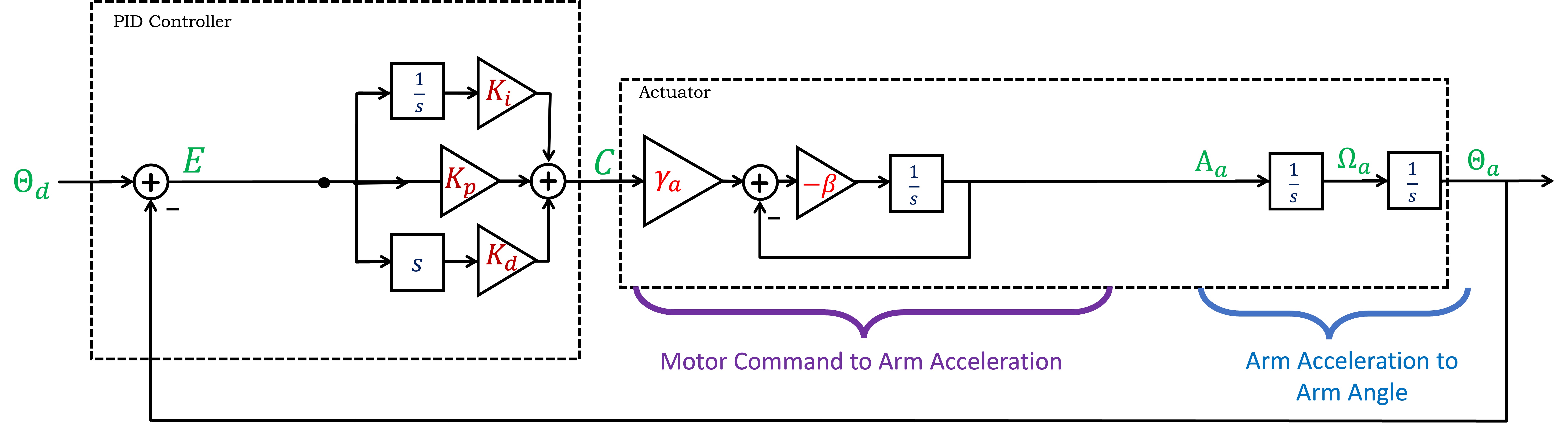
TAKE NOTE THAT WE USE CAPITAL LETTERS when we use system functions. That is, we use capital letters when we substitute, for example,

Blocks described by system functions can be composed by multiplication, and internal feedback loops can be simplified using Black's formula, leading to the following diagram below.

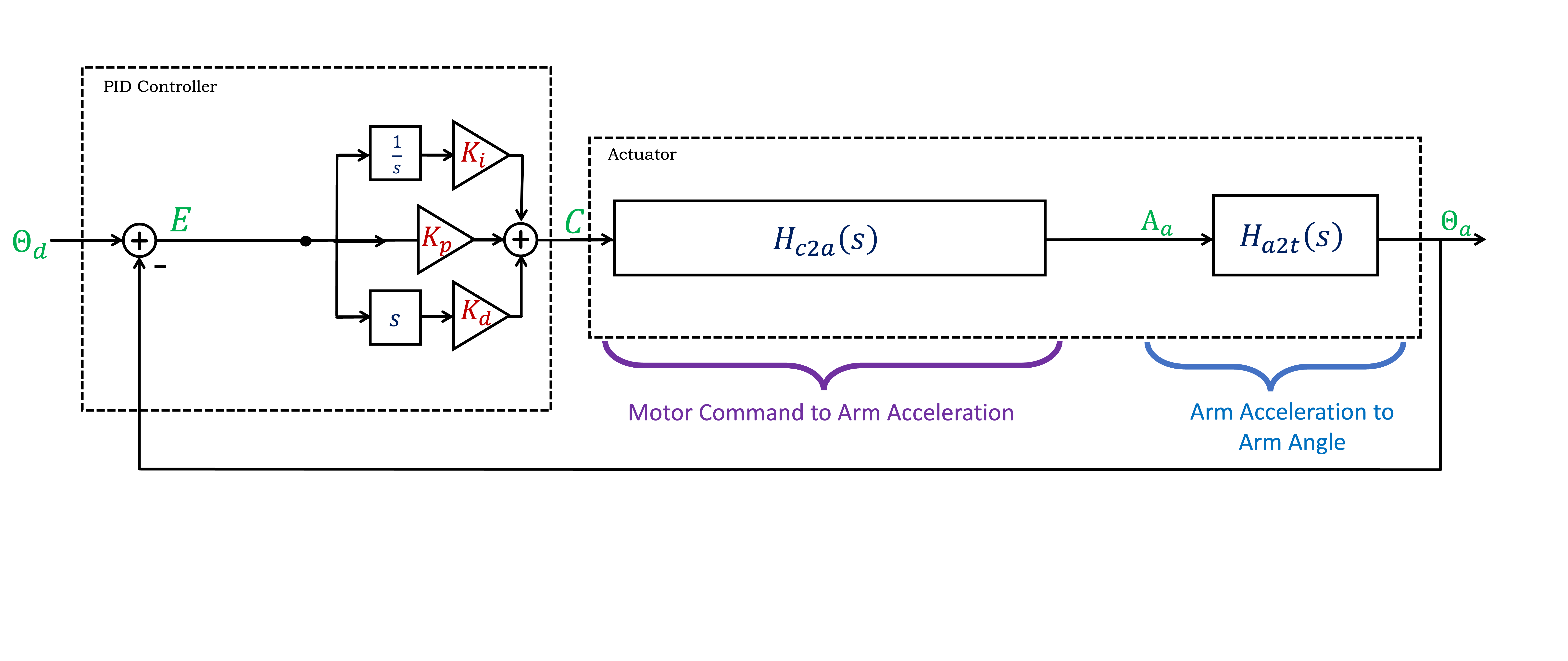
What is the command to acceleration system function, H_{c2a}(s), and what is the acceleration to \theta_a (theta with a "t") system function H_{a2t}(s)? See below if you need a hint.

We can simplify the diagram further by denoting H(s) = H_{c2a}(s) H_{a2t}(s), simplifying the arm block diagram into two system functions, K(s), the controller, and H(s), the actuator, where each is a ratio of polynomials in s, as shown below.

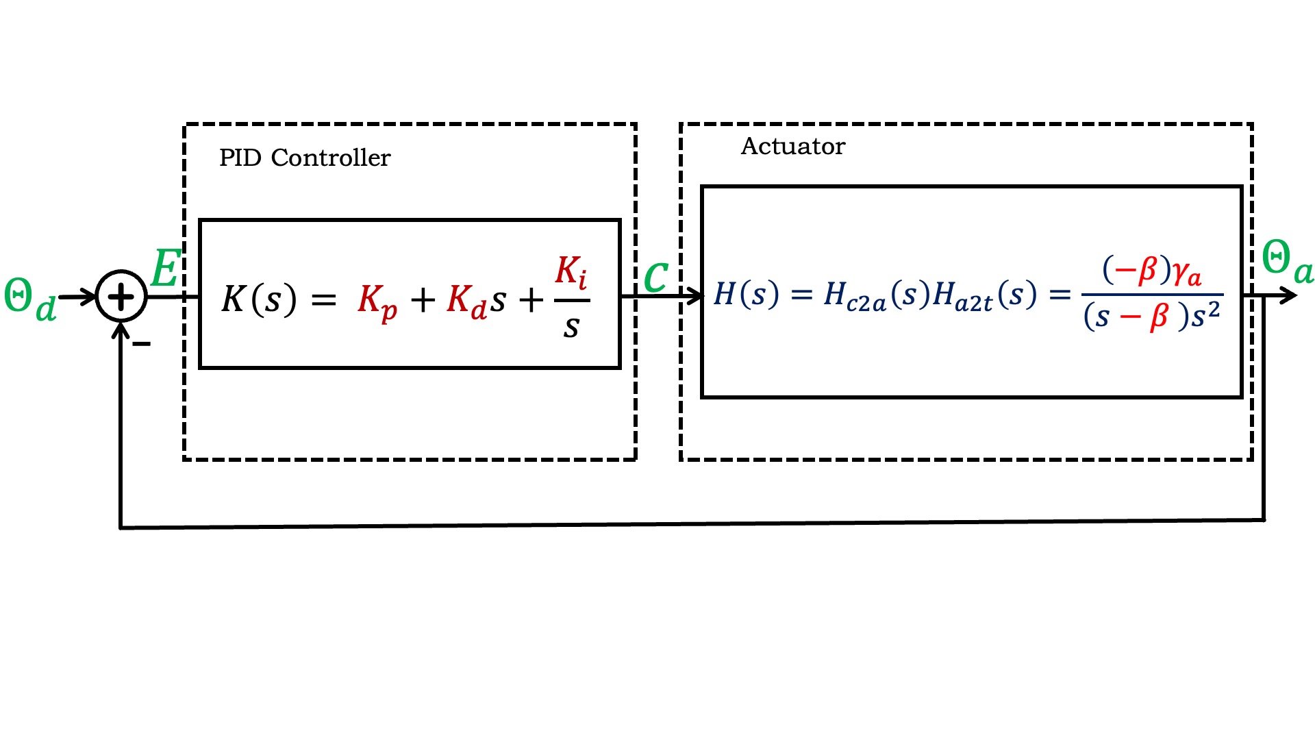
Matlab Tools for CT and Frequency Response.

You can use matlab to manipulate continuous-time transfer functions, but there are a few differences between s- and z-domain manipulation. First, you have to tell matlab to use s as the CT transform variable, by typing

>> s = tf('s')

After that, you can define a CT transfer function. For example, suppose your system is described by a set of differential equations

then where H(s) is the CT transfer function given by

In matlab, if you type

>> H = (1/(s+0.1))*(1/s)*(1/s)

Matlab will response with

H =
 
        1
  -------------
  s^3 + 0.1 s^2

Then if you type

>> pole(H)

matlab will respond with

ans = [0, 0, -0.1000]

as you would expect since in CT, two of your poles are at zero.

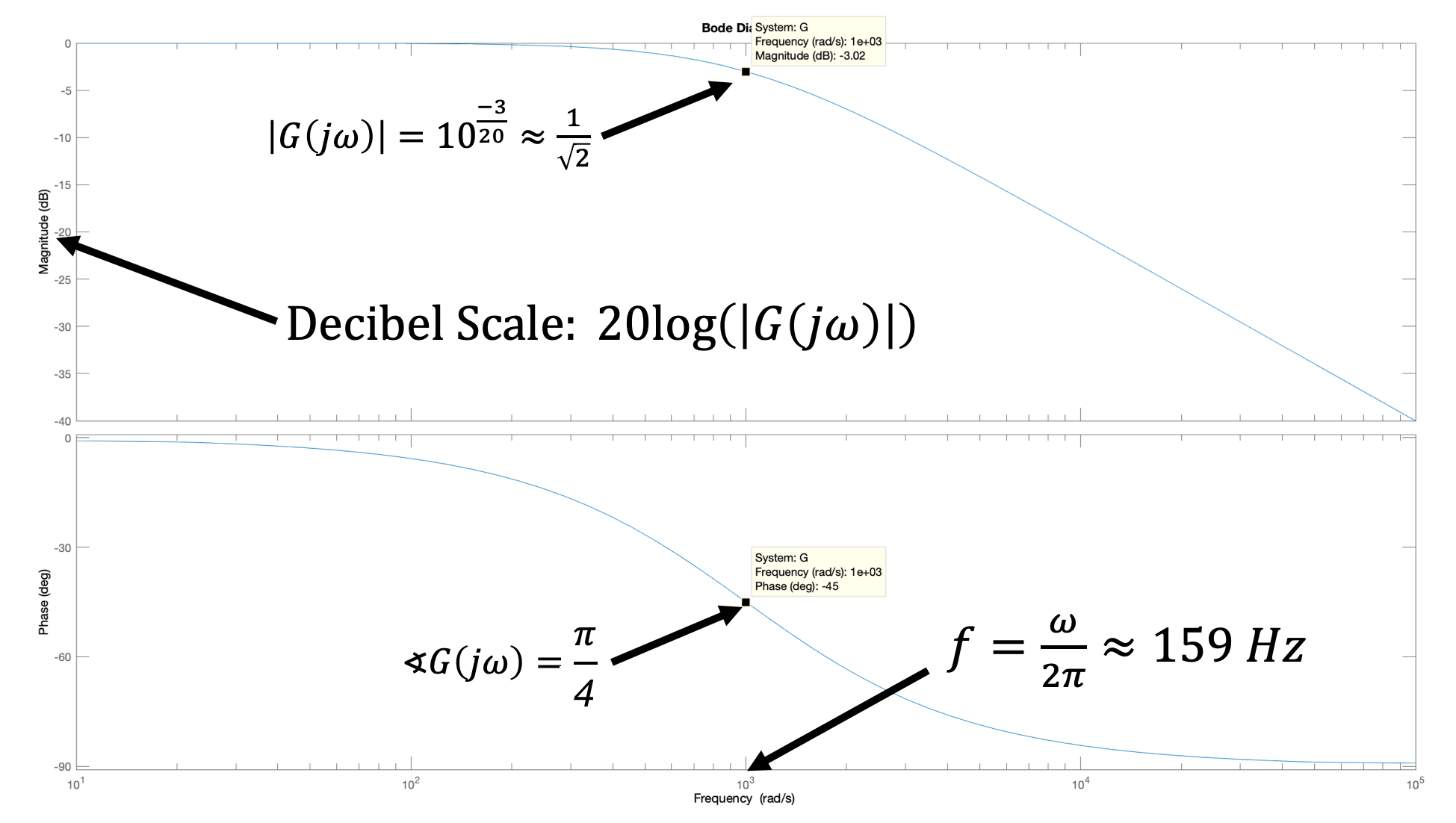
Many of the matlab commands you've used before translate in the obvious way (feedback, step, etc), and we will also make extensive use of the bode command

bode(H)

For example, consider a system with input x(t) and output y(t) described by a first-order differential equation,

where y is the output and x is the input. Suppose we know that x(t) = \cos(\omega t) = \cos(2\pi f t) where \omega is the frequency in radians per second and f is the frequency in cycles per second. Approximately what is y(t) in the limit as t \rightarrow \infty ?

The system function is easy to compute using the techniques described in the prelab, and is H(s) = \frac{1000}{s+1}. If x(t) = u(t), the unit step, then x(t)=0 for t < 0, and x(t) = 1 for t \ge 0. To plot the response to the unit step using matlab, in the command window type (be sure you have defined s to matlab using s = tf('s')).

H = 1000/(s+1)

to define the system function to matlab, and then

step(H)

to plot y(t) given x(t) = u(t). Note that y(t) rises to 1000 with a time constant of one second (about two-thirds of the rise in one second).

The frequency response of this first-order system can be plotted using

bode(H)

If we use unity-gain feedback with this first order system, then

and by using K(s) = 1 in Black's formula, the closed-loop system function, G(s), is given by which matlab can determine for us using the feedback commandt

G = feedback(1000/(s+1),1)

To plot the step response of the feedback system,

step(G)

The frequency response also shows the impact of including the first-order system in a closed loop, as can be seen in the plot generated by

bode(G)

What is different about the open-loop to the closed-loop step and frequency responses?

If we want to determine y(t) given x(t) = \cos{\omega t} in the limit of large t (what we call sinusoidal steady state), we can use the frequency response. That is,

The magnitude and angle of G(j\omega) can be determined from the Bode plot, as as shown in the figure below.

Determining response at a particular frequency from the Bode plot.

Implement the model

Determine an expression for Hc2a.

Determine an expression for Ha2t.

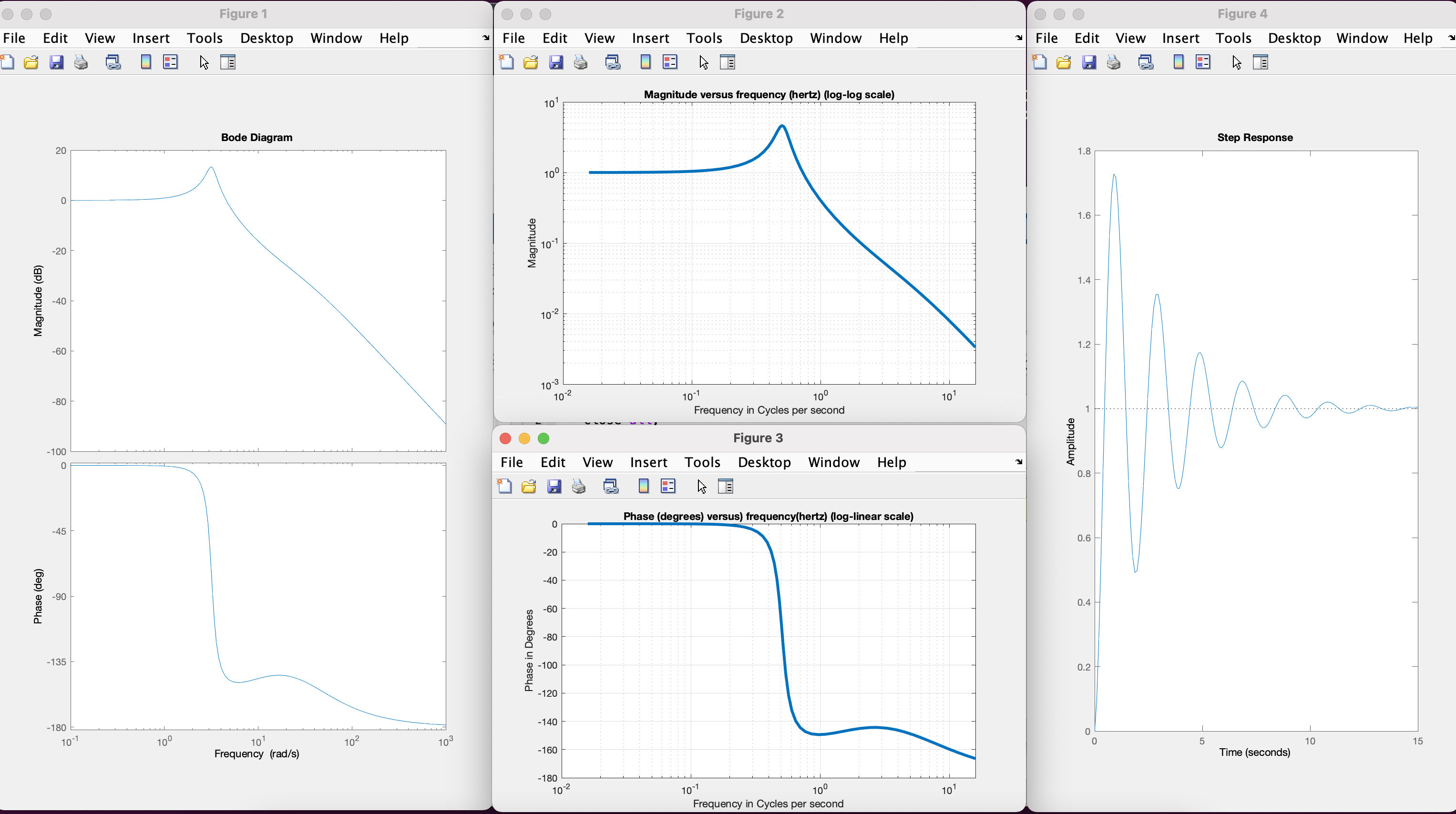
Implement your expressions for Hc2a and Ha2t in the matlab script provided HERE. Running the script should produce plots like the ones below, showing the standard bode plots with the x axis in radians per second, our rescaled bode plots (with bolder lines) in which the x axis is in hertz (cycles per second) instead of radians, and the system step response.

NOTE: We use log to mean a base-10 log, but by default, log in matlab uses natural logarithm (base-e). You can get base-10 log in matlab by using the log10 command.

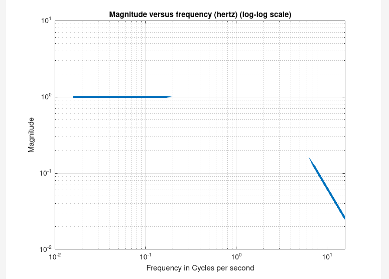
NOTE: For some versions of Linux, the on-line matlab produces disconnected plots for the rescaled plots, like the example below. If you see this, you can just use the non-rescaled Bode plots, but remember that the x axis in those plots is in radians per second, not cycles per second, and must be scaled by 2 \pi.

Test 1: Last week, you found the value of K_d for which your system was barely stable when K_i=4.0 and K_p=0.5. Compare those experiment results with the matlab model. Adjust the parameters, \beta and \gamma_a of the model to get a good match of the step responses of the measurement and model. Also compare frequency responses at a number of frequencies (at least 10).

Test 2: Test the robustness of the model by changing the K's WITHOUT changing the system parameters \gamma_a or \beta. Try the second set of K's from last week: i.e., K_d was set so that the system was barely stable when K_i=0 and K_p=2. Compare step responses as well as the resulting resonance frequencies in the measurement and in the model.

Disturbing Problems

For the propeller arm, we have examined two example disturbances, dropping weight and fanning, as shown in the image below.

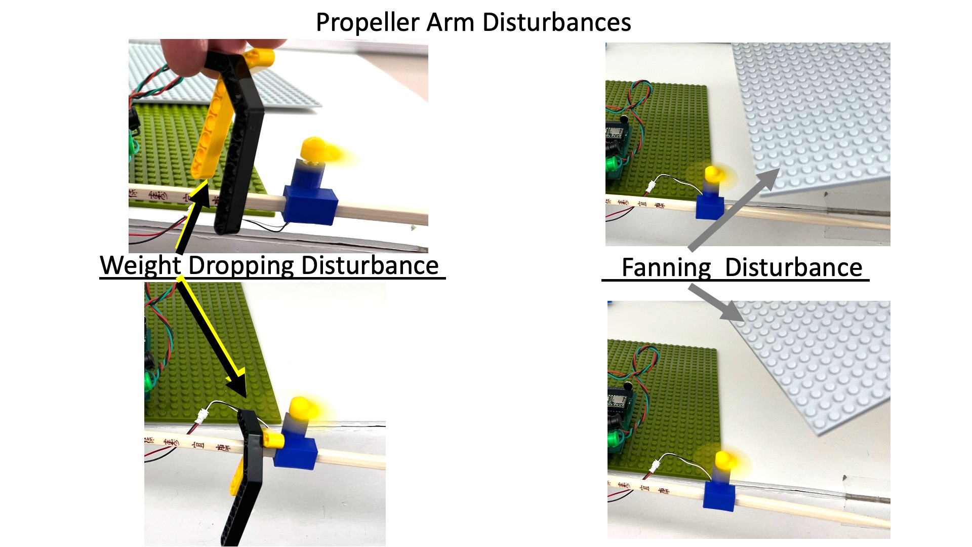
Adding disturbance torques (generated by dropping or fanning) to the abstracted description of arm leads to the image below.

It is simpler to think of the disturbance torques as disturbance accelerations (which is just a rescaling), so it can be added to the CT block diagram, as shown below.

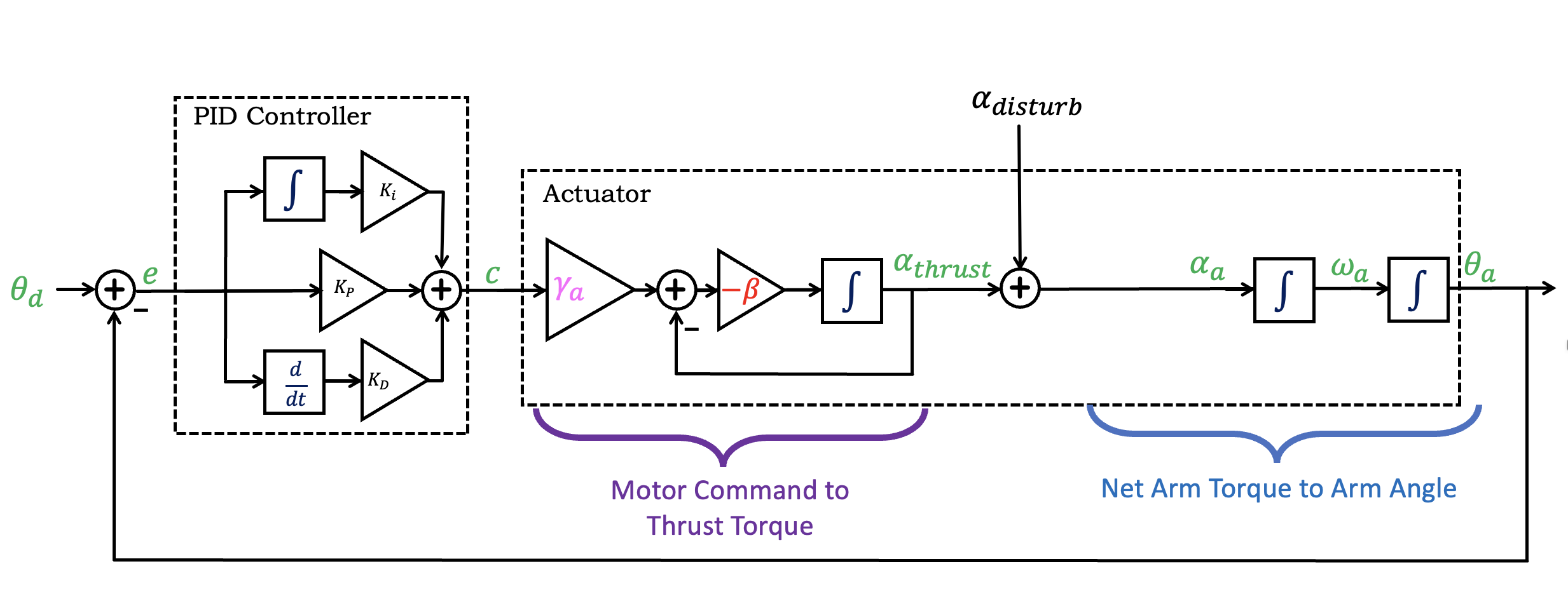
Notice that we introduced \alpha_{thrust}, the acceleration due to the thrust torque generated by the motor-propeller pairs, and added a disturbance acceleration, \alpha_{dist} (as might be generated by "dropping" or "fanning"). Then the sum of two accelerations becomes the arm angular acceleration.

What is the G_{dist}(s), the transfer function from A_{dist} to \Theta_a? To determine that transfer function, we suggest you convert the above diagram using system functions (e.g. K(s), H_1(s), and H_2(s) as we did above). Then, rather than trying to use Black's formula directly, try writing two equations and solving. That is, given

write an additional equation for A_{thrust} in terms of \Theta_d and \Theta_a, and then solve the two equations to determine a relation between A_{dist} and \Theta_a (assuming \Theta_d = 0).

Checkoff 6 - Design a less disturbable controller

Now that you have a calibrated matlab model for your system, and can use the model to plot G_{dist}(j\omega) (to within a scale factor), you can pick K_p, K_i and K_d to minimize the maximum disturbance response. Please do so, and show that your new controller is less "disturbable".