Marginal Maglev Part A: Simplified Model

Quick Reference

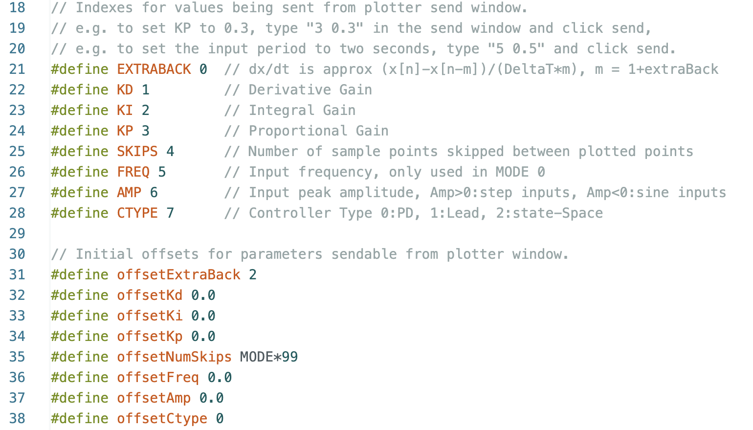
Serial Plotter Send Window Indices and offsets

Links

• Instructions for assembling the Maglev system can be found here.
• Sketch for this lab is here.

Task Summary

Week A

1. Assemble your maglev system (Checkoff 0).
2. Learn about your system using proportional gain only (Checkoff 1).
3. Determine a PD controller that works "sort of" (Checkoff 2).
4. Invert the optical sensor nonlinearity (Checkoff 3).

Week B

1. Determine the parameters for a model of the maglev system (Checkoff 4).
2. Design a CT lead controller and implement it in DT on the Teensy (Checkoff 5).

1) Introduction to Maglev

At the right is a video of LAST TERM's maglev system in action, in which the field produced by a three-coil electromagnet is being controlled to toggle the seperation distance to a floating permanent-magnet-cube "umbrella". For part A of this lab, you will use trial and error to determine a PD controller that keeps a "magnetic umbrella" floating one and a half centimeters below your electromagnet. You will then try toggling the seperation distance to the umbrella, to investigate the stability of your controller. And finally, you will "invert" the nonlinearity of the optical sensor, and show that you can take much larger seperation distance steps with the more linear system.

After spring break, you will finish this lab by taking a more-principled frequency domain approach to designing a FAR MORE EFFECTIVE lead-based controller. The approach will, as always, require a model of the maglev system, a model that you will start developing this week.

1.1) Our Maglev

The above video shows last term's magnetic levitation system in action (we've improved this system every year, and this term's three-coil electromagnet plus sensor nonlinearity inversion is the best ever). You can see two of the three coils for the electromagnet (blue cylinders that surround cores of highly permeable steel), which attracts or repels a cube permanent-magnet (orange) that is part of a floating "umbrella".

The Maglev Actuator and Sensor: Electromagnet, floating "umbrella" (cube magnet, IR reflector, machine screw, and lock nuts), and optical distance sensor inside sensor-rod-and-coil bracket.

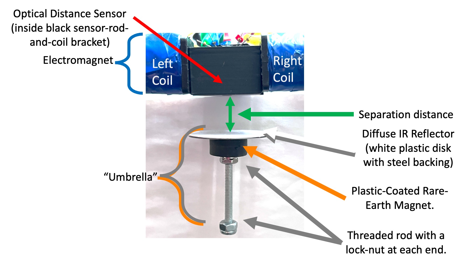
Above is a detailed picture of the electromagnet and the floating "umbrella". The "umbrella" is a plastic-coat rare-earth cube magnet (orange) that holds together a steel-backed white plastic disk and a threaded rod with lock-nut ends. The white plastic disk is a diffuse IR reflector, which makes the distance sensing less sensitive to umbrella tilting. The disk's steel backing has a mirrored surface that is a more efficient reflector, but also more directional, and makes the distance sensing too sensitive to umbrella tilt. The threaded rod with lock-nut ends acts as a tilt stabilizer, much like the tail on a kite.

The electromagnet is driven by a feedback control system that senses the distance between the umbrella and the electromagnet, and adjusts the electromagnet's field to hold the umbrella "floating" about a half inch beneath the electromagnet.

In this lab you are going to put together this electromagnet, attach an optical distance sensor, calibrate your setup, model your levitation system, and then design the controller that holds the "umbrella" floating in space.

Technically, calling this task "Maglev" is a misnomer. This is not magnetic levitation, as we are not causing the object to "rise", but rather, the object is "hanging". But there is no combination of magnet and hang that sounds as cool as Maglev. Please forgive us our trespasses.

1.2) Maglev Demos

We've used a number of different coil magnet arrangements for this magnetic levitation lab, but regardless of the implementation details, the issue of determining a nominal command (using the potentiometer) has required some experience. In this first video (using an earlier term's electromagnet), we give you some hints about how to adjust the potentiometer while trying to float the magnet. It can be a little tricky, as the "blooper" video shows. The other videos are just for fun, and show a few other magnet topologies.

1.2.1) Two challenging levitation demonstrations (using a nine-volt power supply)

DO NOT TRY AT HOME. Rare earth magnets are dangerous! They are brittle, and when they slam into each other, they send shards of metal flying. We give you the small disc magnets for a reason!

1.2.2) Videos from Students and Staff.

2) Assemble the Maglev System

Complete the assembly of the maglev system:

1. Instructions for assembling the maglev system can be found here.
2. Sketch for this lab is here.

Follow the instructions at the end of the assembly guide for coil checking and calibrating your system.

3) The Magnetic Levitation System and its Forces

In our magnetic levitation system, a plastic-coated rare-earth magnet is "floating" about half an inch below the bottom pole of the electromagnet. A diagram of the electromagnet/permanent magnet system, with the forces noted, is shown in the figure below.

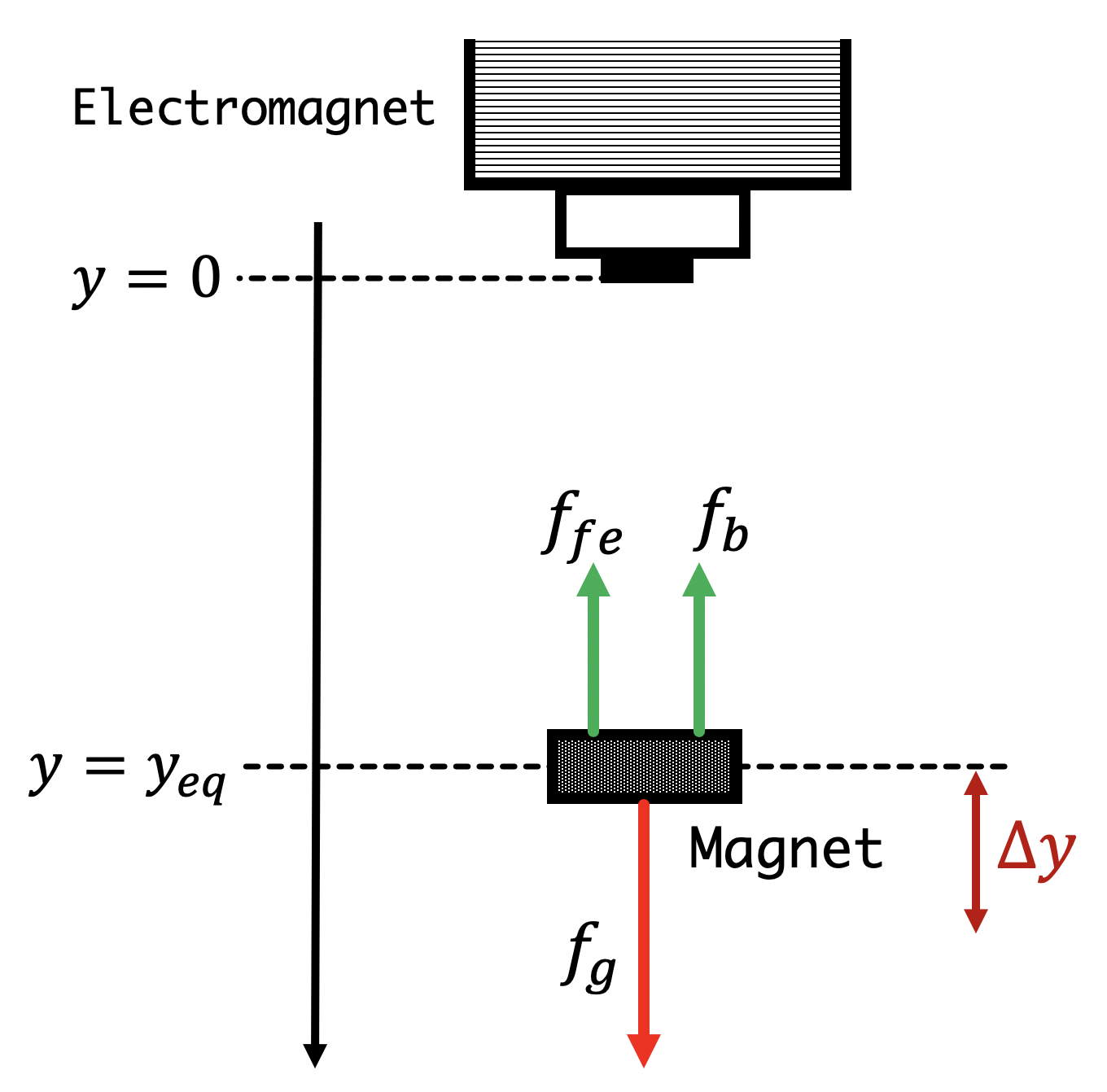
In the above diagram, a magnet is "floating" at a position y_{eq} beneath the bottom pole of an electromagnet, and our job will be to adjust the field produced by the electromagnet (by adjusting voltage across the electromagnet's coil, c(t)) so that the magnet is held stable at that position.

To design the controller, we could start by developing a model of the net force, a sum of a position-independent gravity force, f_g, and the position dependent forces of attraction: the force of attraction between the floating magnet and the electromagnet's iron core (in our case a steel bolt), f_{fe}, and the force due to the electromagnet's field, f_b. After determining analytic expressions for each of the individual forces as a function of position, y, we could derive a formula for the total force, f(y) = f_g + f_{fe}(y) + f_{b}(y). Then armed with f(y), we could find the force-balance equilibrium position, y_{eq} such that f(y_{eq}) = 0. Finally, we could determine how to drive the electromagnet, as a function of the perturbation from equilibrium, \Delta y shown in the above figure, so that the magnet is pushed back to y_{eq}.

The physical modeling is possible, but a few measurements will get us the information we need. Assume the magnet starts at y_{eq}, and the zero net force is perturbed by some \Delta f. Then the net force on the magnet is no longer balanced, and the magnet will accelerate away from equilibrium. That is, the perturbation in force can be related to the perturbation in position by

where \Delta y is perturbation from y_{eq} (as shown in the above diagram) due to the force perturbation, and \gamma_{da/df} is the proportionality constant relating changes in acceleration to changes in force.

Now, what could perturb the force? If the magnet's position is perturbed, moving it either closer to, or further from, the electromagnet and its iron core, then both magnetic forces, f_{fe} and f_b, will be perturbed. We can also perturb how we drive the electromagnet, which will produce a perturbation in the electromagnet's measured field, \Delta b, and in turn, perturb f_b, the force on the floating magnet. If the perturbations are small enough, we can linearize the relation between force perturbation and perturbations in position and electromagnet field

Combining the two relations, we arrive at an equation of motion about the equilibrium point y_{eq},

From the algebra (or the chain rule), which indicates that the perturbation in magnet acceleration due to perturbations in position is a product of the acceleration's sensitivity to perturbations in force multiplied by the force's sensitivity to changes in position.

Similarly,

which indicates that the perturbation in magnet acceleration due to perturbations in electromagnet field is a product of the acceleration's sensitivity to perturbations in force multiplied by the force's sensitivity to changes in electromagnet field.

It may seem unimportant to establish relationships between constants whose values you are unlikely to learn. Nevertheless, we have learned the form of the transfer function relating the perturbation in position to the perturbation in electromagnet field,

and we will see later how to use that to assist in design.

For now, let us see if we can estimate \gamma_{da/dy} for our system. Suppose you held a disk magnet underneath the electromagnet, and that you are setting the electromagnet's field to a fixed value. Perhaps you could adjust things so that the upward pull of the total magnetic attractive forces is nearly equal to downward pull of gravity. If you then increased the electromagnet's field a little bit, and let go of the disk magnet, what would happen? What does that tell you about the sign and order of magnitude of \gamma_{da/dy} ? Answering the following question may help you better understand what will happen.

3.1) A very related example.

The following are six step responses, four of which are associated with the transfer function for one of four different values of \gamma, 1, -1, 25, -25. For each plot, give the associated \gamma and the natural frequencies (in any order) as a python list. If the plot could not be a step response for H(s), enter a list of three zeros [0,0,0].

Note: you must enter the answer as a Python list for grading to work, and please use j=\sqrt {-1} and enter decimal representations in place of fractions wherever necessary. For example, \frac{7}{8}+\frac{1}{2}j is entered as 0.875+0.5j, and a value for \gamma followed by two natural frequencies would be [17.6, 0.875+0.5j, 0.875-0.5j]. Finally, if you want to enter -j or +j, please enter -1j and 1j.

3.2) Proportional Gain Controller

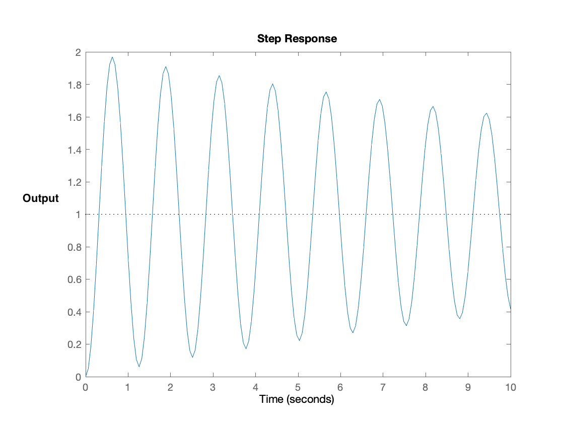
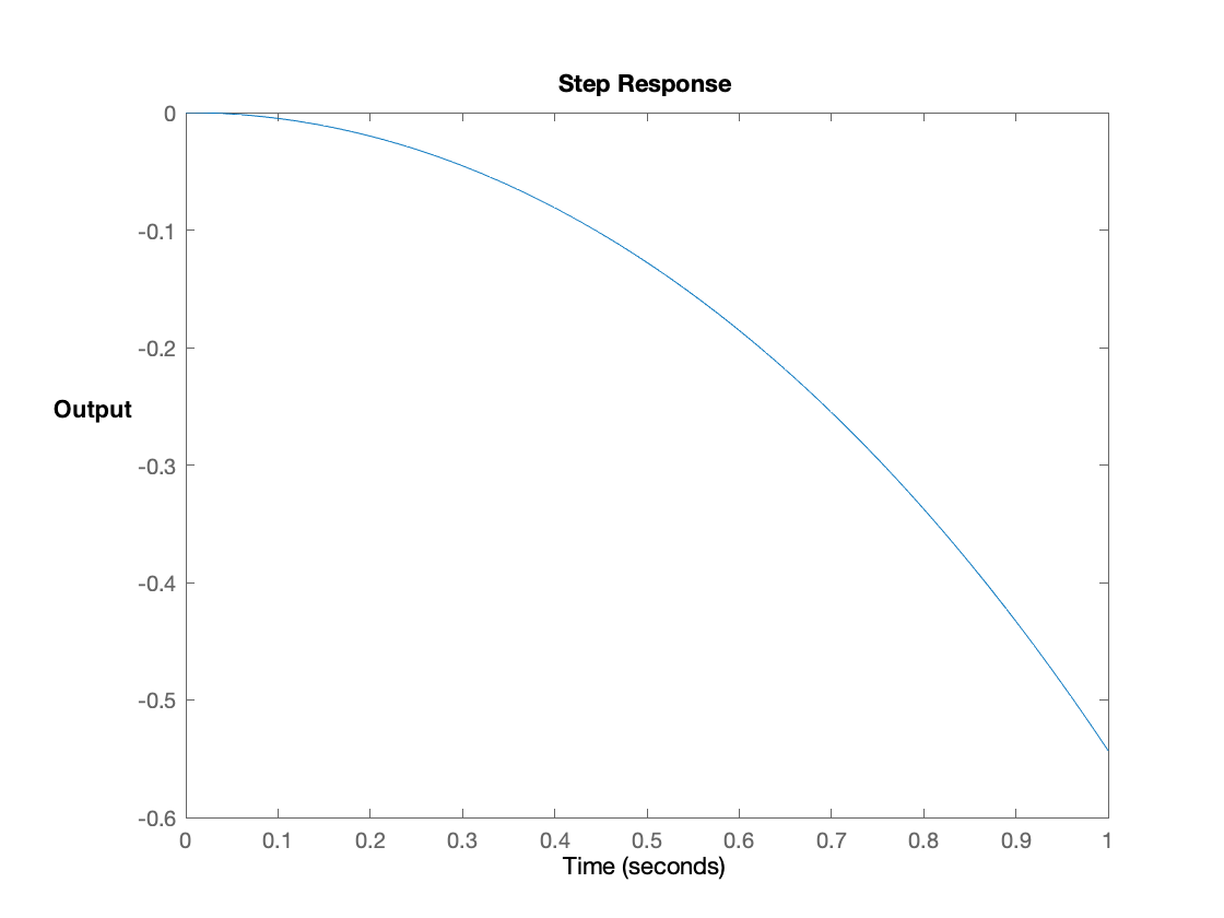
As a first step in designing the controller, we will determine a proportional feedback gain K_p as follows. Start by using the potentiometer to set the nominal field so that it approximately cancels the gravitational force on the umbrella when the umbrella is at its nominal zero location, which is 1.5 cm from the optical sensor. Then set K_p to be large enough to repel the umbrella when it is too close to the optical sensor and attract it when it is too far away. Notice that the feedback system with just proportional gain will be unstable, but unlike the open-loop system above, its behavior should be oscillatory (see the video at the end of the assembly guide). There is no need to be precise. This step is intended to qualitatively provide insight into the design of a useful model.

3.2.1) Testing

The end of the assembly guide shows how to calibrate and test your maglev system. Please be sure to test that the optical distance sensor has the correct range and offset, that the three electromagnets are aligned, and to check the sign of, and effect of, the proportional gain.

Once you have tested your system, watch the last video in the assembly guide and try to get your system to oscillate by finding a good K_p and a good setting for the nominal command.

Be sure to watch out for a sign error! If the electromagnet more strongly attracts the umbrella as the separation distance shrinks, instead of repelling it more forcefully, flip over the cube magnet and try again.

3.2.2) Modeling

Once you have determined a sufficiently high gain to produce oscillation, you can try analyzing the feedback system. Unlike the propeller arm, you will not be able to get a completely calibrated model, but you can learn enough to constrain your search for a good controller.

To begin, lets simplify the problem by assuming we can directly measure the perturbation in separation distance, \delta y(t), and directly control the perturbations in the electromagnet's field, \delta b(t). Assuming the coil field changes instantly with changes in controller command is analogous to the instant thrust model we used with the propeller arm. When we include a model for the dynamics relating the controller command to the generated force (either thrust or magnetic attraction/replusion), we often refer to including the "electronic pole".

For now, we will ignore the electronic pole, and model the levitation system as

and that your proportional gain feedback system generates a field such that where K_{p} is a proportional gain, and \Delta Y_d (s) is the desired change in position (equal to zero if we want to hold the floating magnet in one position).

A proportional-gain feedback diagram for the maglev, with electronic pole ignored (NOT USEFUL FOR DESIGNING COMPENSATOR).

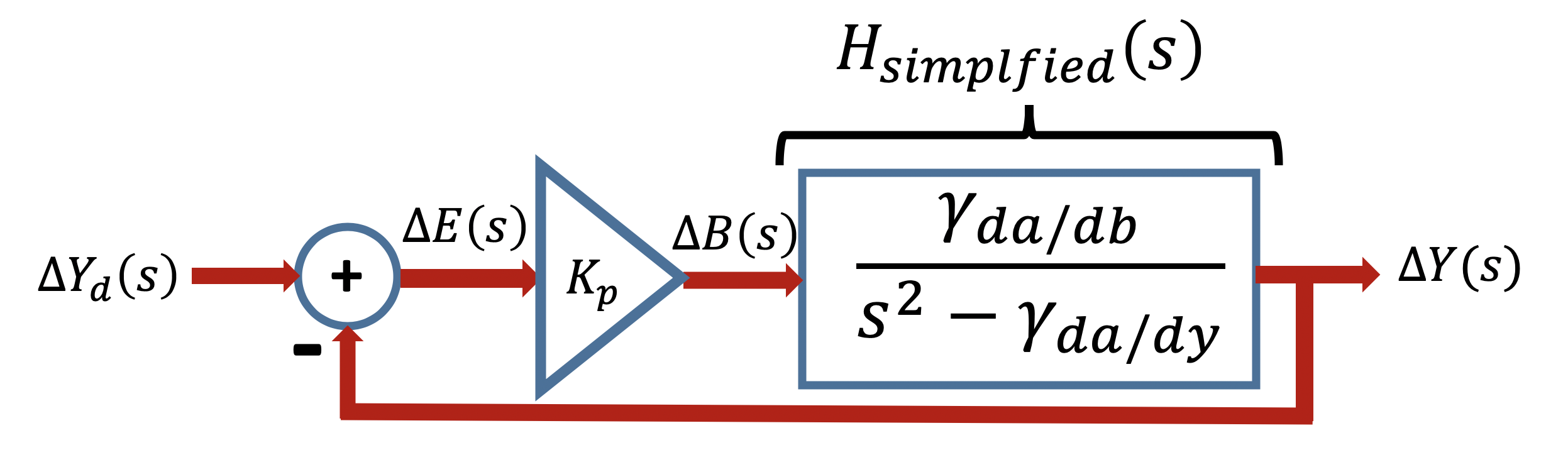
Can you determine the closed-loop transfer function from \Delta Y_d to \Delta Y for this simplified model of the proportional-gain feedback system? And based on your experiment, where are the closed-loop poles (are they real, imaginary or complex)? What can you say about the sign of

given the behavior you noticed during your experiment, and given what you know about the closed loop poles of the proportional-gain-only feedback system?

4) PD Control and Step Responses

For this second checkoff, we would like you to find a value for K_p and K_d, a PD controller, so that the umbrella remains suspended beneath the electromagnet. You should also be able to track a \frac{1}{2} hertz square wave for an amplitude of at least 0.02, and probably almost 0.1 (set using send window, "5 0.5", "6 0.1"). But, don't expect to follow the step exactly, or to hang on for long, like in the video below (using LAST TERM'S SETUP).

If you are having trouble tracking a square wave, try setting PSMOOTH on line 49 in the sketch to 0.95.

5) Inverting the Optical Sensor Nonlinearity

As the picture below makes clear, the optical sensor quite nonlinear. Starting with the umbrella in the zero position (as set by the spacer), the sensor reading is more than eight times more negative as the umbrella moves 1.5 centimeters closer to the sensor than when it moves 1.5 centimeters further away.

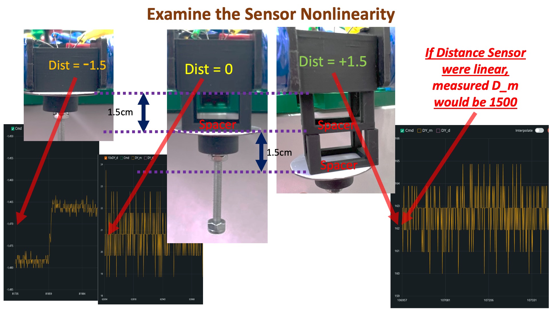
We are sensing distance optically. Specifically, our sensor generates an infrared light beam and then senses the strength of the reflected light. We then determine distance by offsetting and scaling the sensor output, though since the sensor signal is larger when the umbrella is closer, our equation for distance has a negative sign. You can see this by examining equation on line 177 in the sketch,

float deltaY = SensorOffset - SensorScale*sensVal;

where deltaY is the distance in centimeters (the plotter scales by ten thousand to convert centimeters to microns).

A better model for the relation between the sensor output and umbrella distance is to assume that the sensor output is INVERSELY PROPORTIONAL TO DISTANCE. That suggests that we should offset and scale the INVERSE of the sensor output to determine distance, as in the Teensy equation

float deltaY = SensorOffset + SensorScale/sensVal;

Notice that we are using \frac{1}{sensVal} in the above. And of course, when we change to using \frac{1}{sensVal}, the values for SensorOffset and SensorScale will change completely. Notice, for example, that the formula does not have a negative sign (do you see why)?

We know that the sensor value is nonlinearly related to umbrella distance, and we know that linearizing a nonlinearity about a nominal point can interfere with linear control (unless distances from the nominal are all vanishingly small). But if we know the nonlinearity, as we do in the case of the optical sensor, we can remove it rather than linearizing it. Try implementing and calibrating the

formula in the Teensy sketch. Does the new approach give you more reasonable values for the umbrella positions of -1.5 and +1.5 centimeters away from the umbrella zero position? Note that you have three calibration positions, at -1.5, 0, and +1.5, but only two parameters, SensorOffset and SensorScale, so you will not get a perfect match.

Once you MOSTLY eliminate the sensing nonlinearity, does your PD controller perform better? Do you expect it will perform better for small steps? Larger steps? Try it and see!