Marginal Maglev Part B: Lead Design

Measuring "time."   The time dT between adjacent points plotted in the plotter window is programmable. In mode 1, dT is equal to (99+1+SKIPS)*0.0001 seconds. If you do not enter a value for SKIPS, or if you enter SKIPS = 0 (by typing 4 0), then dT is 0.01 seconds. If you enter SKIPS = -50 (by typing 4 -50), then dT is 0.005 seconds. In mode 0, the time difference is given by (1+SKIPS)*0.0001 seconds, i.e., the offset value is 0 instead of 99.

Quick Reference

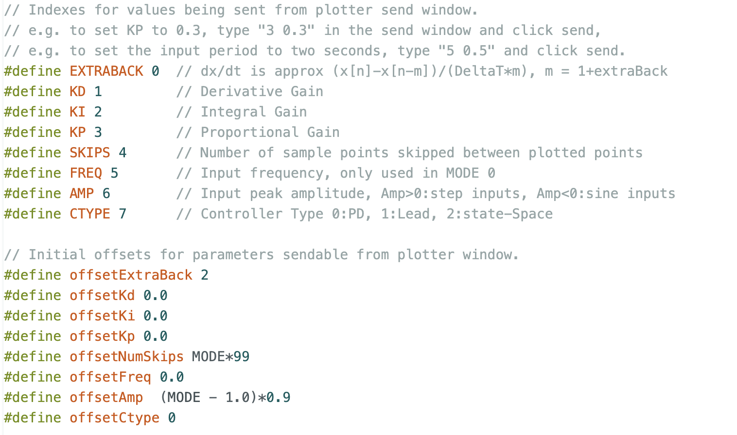
Serial Plotter Send Window Indices and offsets

Links

• Instructions for assembling adding the magnetic field sensor to your maglev system can be found here.
• Sketch for this lab 6310_MAGLEV_SP24.zip

Task Summary

1. Complete last week's lab FIRST!.
2. Download the sketch.
3. Check coil current directions for consistency with a compass.
4. Recalibrate the sensor scale and offset.
5. Add a magnetic field sensor, as described at the end of the maglev assembly guide (see link above).
6. Calibrate the controller-command to coil-current model (Checkoff 1).
7. Calibrate the system model, and demonstrate model-measurement matches(Checkoff 2).
8. Use the model to design, and then test, a lead controller (Checkoff 3).

1) What to Expect.

In the two videos below, we show two "working" maglev systems, one using a PD controller, on the left, and one using a lead-based controller, on the right. In the video on the left (the PD controller), you can see that the command (in green) is rapidly jumping up and down between its most positive and most negative values. This noisy command leads to noise in the umbrella position, as you can see by comparing the plot of the desired and the measured umbrella position (in red and blue respectively), or by examining the actual umbrella motions. The situation is quite different in the video on the right (the lead controller). The command (in green) has some noise, but far less than the PD-case noise. Note also that the response, in blue, tracks the desired response more cleanly (as you can see from the measurements plotted in blue, or by watching the umbrella). The difference is not subtle!

Notice also that for both controllers, the desired position (in red) is a smoothed square wave, generated by setting Psmooth near line 50 in the sketch to 0.999. You will investigate reasons for using a smoothed square wave at the end of this lab, but DO NOT SMOOTH THE INPUT SQUARE WAVE WHILE CALIBRATING YOUR MODEL! The maglev system's response to those rapid transitions can be very informative.

2) Review of Part A

In the last lab, we constructed the Maglev system that suspended an "umbrella" (a cube magnet with a white plastic diffuse reflecting top and a threaded rod tail). As a reminder, we:

1. Used black 3-D printed spacers to
   • calibrate a nonlinear function for accurately estimating the distance between the umbrella and the electro-magnet from the optical sensor signal and
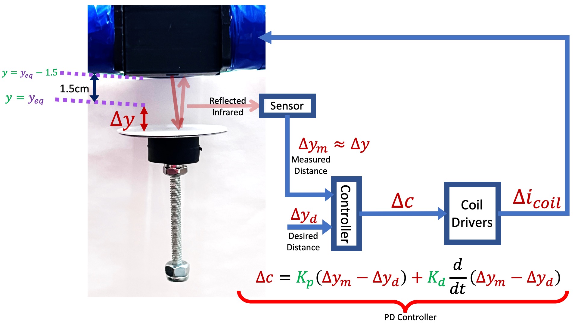
   • establish an umbrella equilibrium position, y = y_{eq}, 1.5 centimeters below the electro-magnet;
2. linearized, about y_{eq}, the relation between umbrella acceleration and electro-magnet coil current;
3. investigated proportional feedback stability using the linearized model, assuming coil currents instantly track changes in Teensy command;
4. determined gains for a PD controller to "float" the umbrella.

Before we begin part B, designing a lead controller, we will need an more accurate model of our system. So let us we review (by picture) what was investigated in part A.

2.1) Umbrella Forces

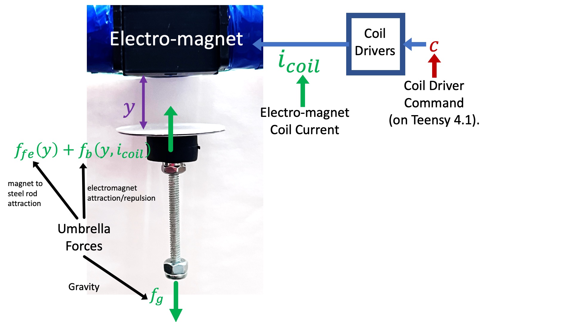
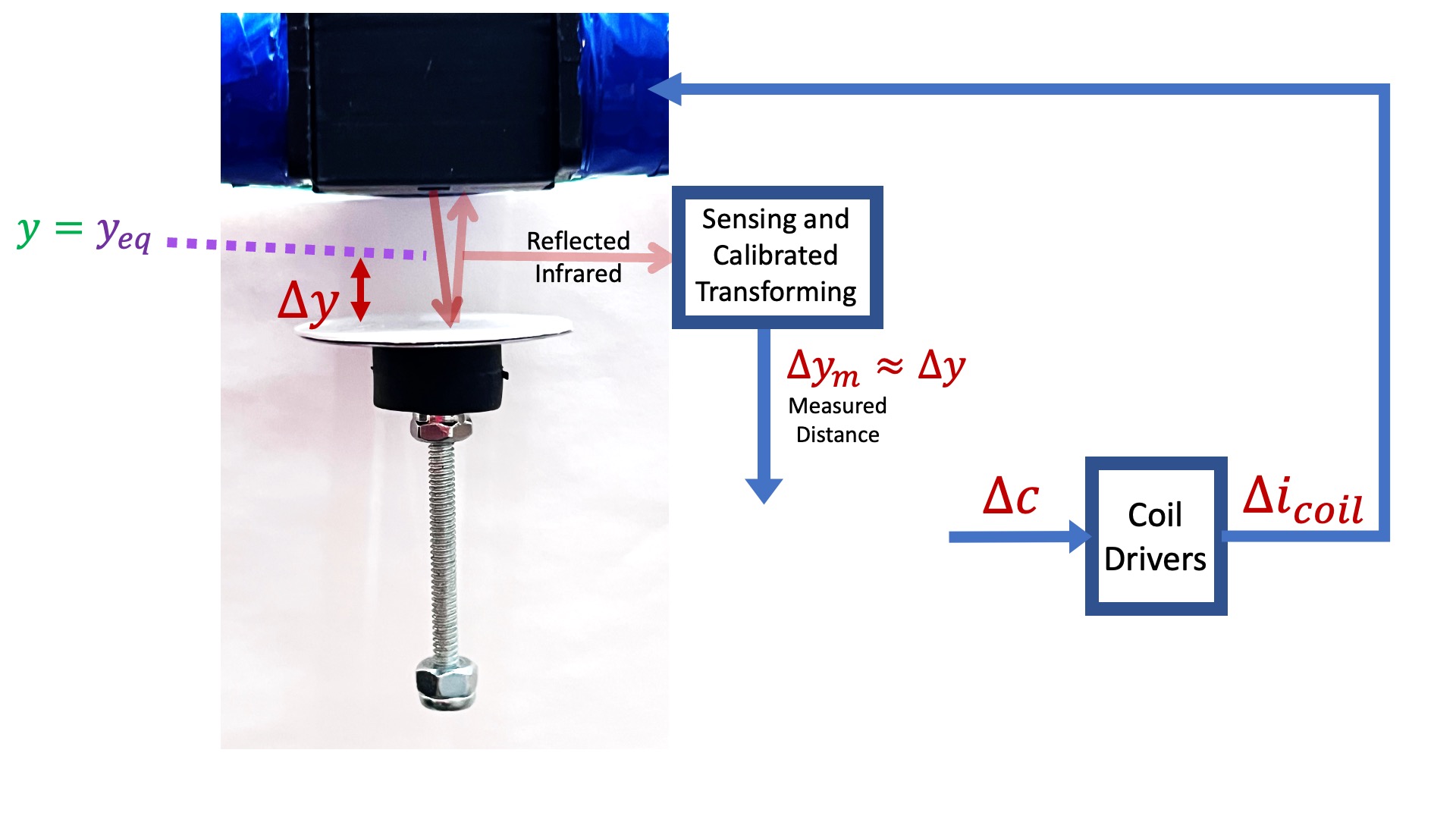
In the figure above, we note the forces acting on our cube-magnet "umbrella": a position-independent gravity force, f_g; a position-dependent force attracting the cube magnet to the electro-magnet's steel core, f_{fe}(y); and a coil-current and distance-dependent attracting/repelling force between the cube magnet and the electro-magnet f_b(y,i_{coil}). Recall that for our solenoid-type electro-magnets, magnetic field is proportional to coil current, making them interchangable up to a scale factor.

2.2) Equilibrium Position

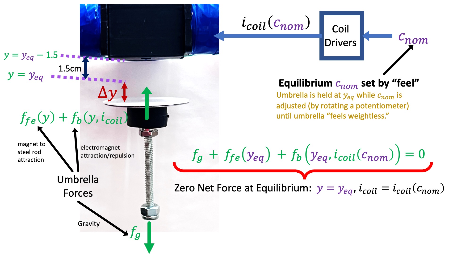
In the above figure, we note the definition of \Delta y , the distance from the force-balanced equilibrium position y = y_{eq}.

2.3) Linearizing

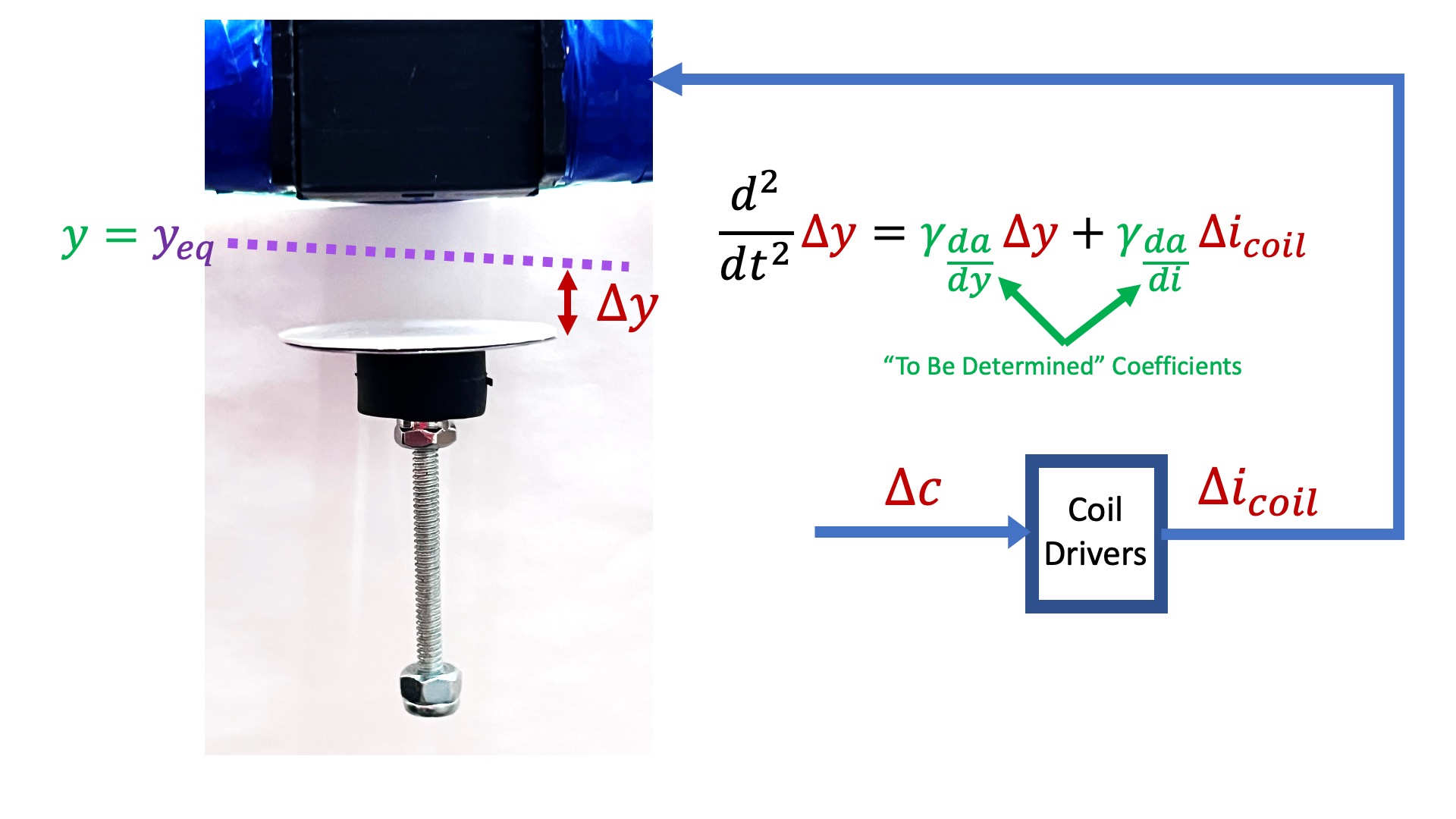
Note that, compared to the previous lab, f_b is defined as being dependent on the electro-magnet's coil current rather than its field. As a result, our linearized model has \gamma_{\frac{da}{di}}, which relates perturbations in coil current to perturbations in umbrella acceleration, along with \gamma_{\frac{da}{dy}}, which relates perturbations in umbrella position to perturbations in umbrella acceleration.

2.4) Position Sensing and Transforming

In the previous lab, we calibrated a nonlinear relationship between \Delta y and the optical distance sensor voltage (see lines 177, 178 the in Teensy sketch). Please be sure to recalibrate that relationship.

2.5) PD Feedback Control

Previously we used an ad-hoc approach (we guessed) to finding a PD controller that levitated the umbrella. With that PD controller, we can make measurements that help us improve our model of the maglev system. Once we have a model, we can use the phase margin concept to design a better controller.

3) The Abstraction Process and Today's Tasks.

Perhaps it is helpful to review the abstraction process before we delve into estimate model parameters. That is, how did we arrive at a transfer function description of the coils, magnets, umbrella, and controller that comprise the maglev system?

3.1) Functional Diagram

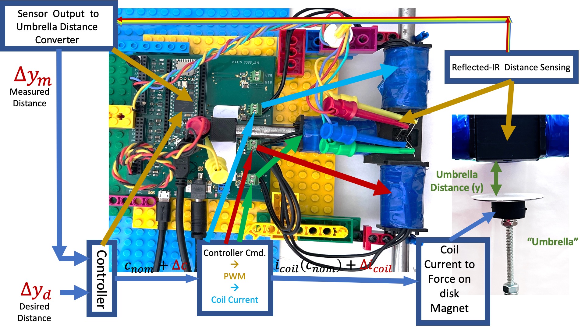
In the above diagram, we note the connections between the abstract blocks we will manipulate mathematically and the physical system.

3.2) Block Diagrams

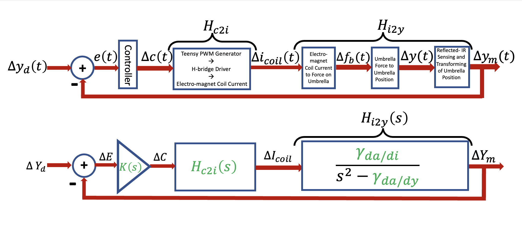
The above block diagrams show two more steps in process of abstracting the physical system into a composition of transfer functions. Note a key decision imbedded in the diagrams, a choice of variables. That is, we chose certain physical variables in our perturbation model, \Delta y_m, \Delta i_{coil}, and \Delta c. In general such choices are not unique, and are often based on intuition rather than more formal reasoning.

The transfer function abstraction clarifies (in green) what we are missing: the two parameters in the transfer function relating coil current to umbrella position; H_{c2i}(s), which relates controller command, c, to coil current, i_{coil}; and of course the improved controller, K(s).

3.3) Today's lab

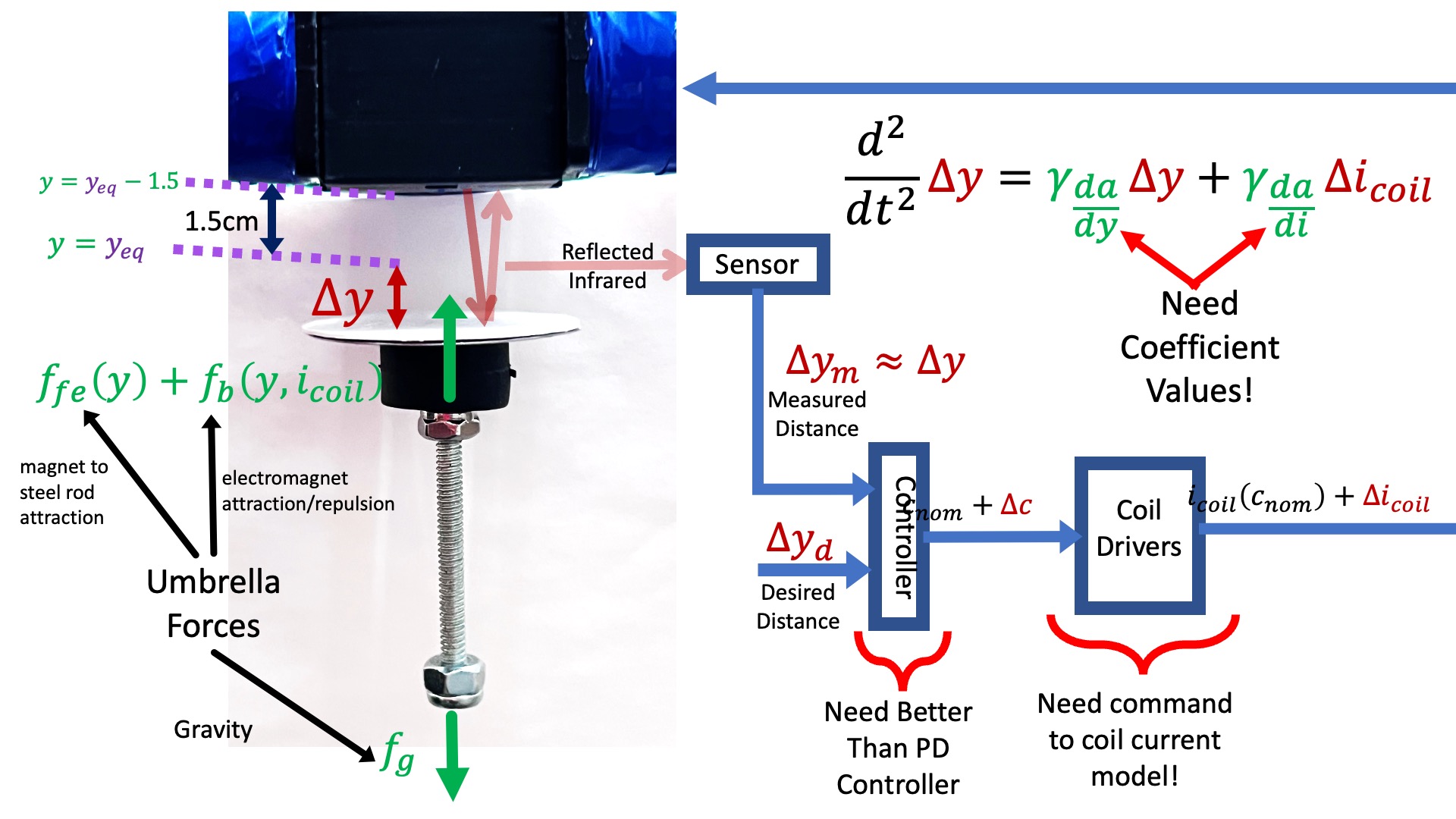
The figure above is a summary of our tasks for today's lab. We will need to

1. Determine a controller-command to coil-current model,
2. Estimate coefficients for the model,
3. Use the model to design a better controller.

4) Command to Current Modeling.

The electro-magnet is made up of three wire coils surrounding three steel cores, each of which is driven by its own H-bridge driver. Together thay generate the field that either attracts or repels the umbrella's cube magnet.

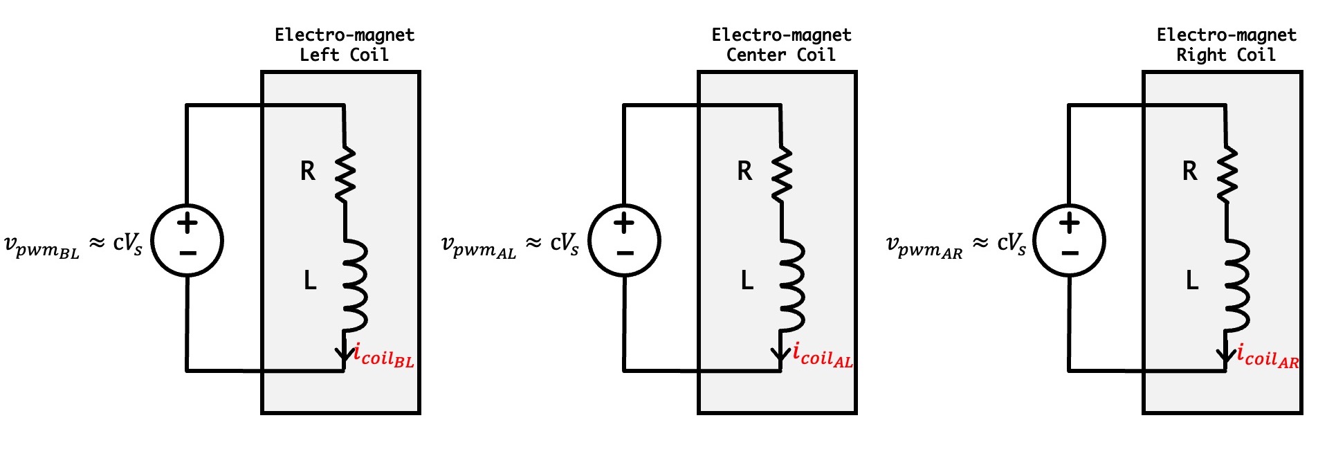
In the above circuit-ish diagram of the three-coil maglev electro-magnet there are:

• three voltage sources, v_{pwm_{BL}}, v_{pwm_{AL}}, and v_{pwm_{BR}}, which model the three H-bridge coil drivers and
• three series resistor-inductor (RL) combinations, which model the inductance and wiring resistance of each of the three coils.

As a result, there are three coil currents, i_{coil_{BL}}, i_{coil_{AL}}, and i_{coil_{BR}}, which are, as we noted before, proportional to each coil's field.

In our case, the three voltage sources have identical voltages, given by the product of the power supply voltage, V_{ss} (five volts in our case) and the Teensy command, -1 < c < 1. So if c changes instantly from -1 to 1, the three voltage sources change instantly from -5 to 5 volts, but the non-zero coil inductance prevents the coil currents from changing instantly.

Sound familiar? Recall that when we changed the voltage across the propeller motor, the thrust did not change instantly.

4.1) The R-L Circuit

Since all three voltage sources are equal to V_{ss} c, if we assume all three inductors and resistors are equal, then all three coil currents will be equal. So we'll just analyze one R-L circuit.

From the circuit model, the voltage across the resistor plus the voltage across the inductor must equal the source voltage. Using the inductor and resistor constituitive relations,

or

Assuming c(t) = Ce^{st} and i(t) = I_{coil} e^{st}, we can determine the transfer function relating the Teensy command to the coil current,

4.2) Abstracting

We can abstract the circuit elements from the relation between coil current and Teensy command, to see that there are only two parameters in the relation,

and where \lambda_E is the natural frequency, or pole, for the electromagnet, and \gamma_{\frac{di}{dc}} is a the proportionality constant.

The transfer function relating Teensy command to field in the electromagnet is then

with only two parameters to determine.

4.3) Measuring

Since our model corresponds to a first-order CT system, when we excite the system with a step, we get a response whose steady-state is easily related to our model's scale factor \gamma_{\frac{di}{dc}}, and whose rise time is inversely proportional to our model's natural frequency \lambda_E. And when we excite the system with a sinusoid of frequency \omega (in radians/second), if |\omega| = |\lambda_E| then the sinusoidal-steady-state response will be phase-shifted 45 degrees from the excitation, and will be a factor of \frac{\sqrt(2)}{2} smaller than the amplitude of the sinusoidal-steady-state response for |\omega| is much lower (e.g. \omega < 0.1 |\lambda_E|).

If you set the MODE on line 10 of the Teensy sketch to 0 (which is only for testing the coil, NOT FOR MAGLEV), upload the sketch, and set the frequency (by typing 5 10 to set the frequency to 10 hertz, for example), you should see the sinusoidal command, c(t), and the coil current response, i_{coil}(t). You can then change the frequency (though you may have to change the number of skipped points in the plotting to see the sinusoids clearly, try typing 4 2 in the send window). You can also plot step responses, by changing the amplitude of the input (try typing 6 1.8 in the send window), that will change the preset value of the amplitude from -0.9 to 0.9, and it will switch to square waves). Be sure to use a low enough square wave frequency so that the coil current achieves quasi-steady-state.

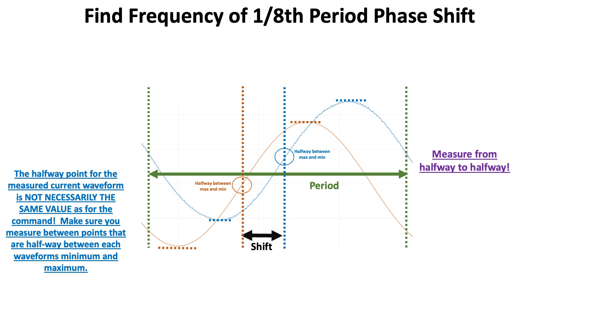
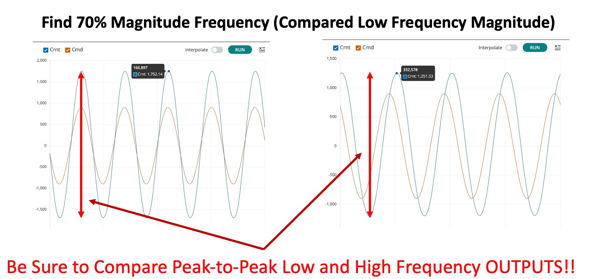
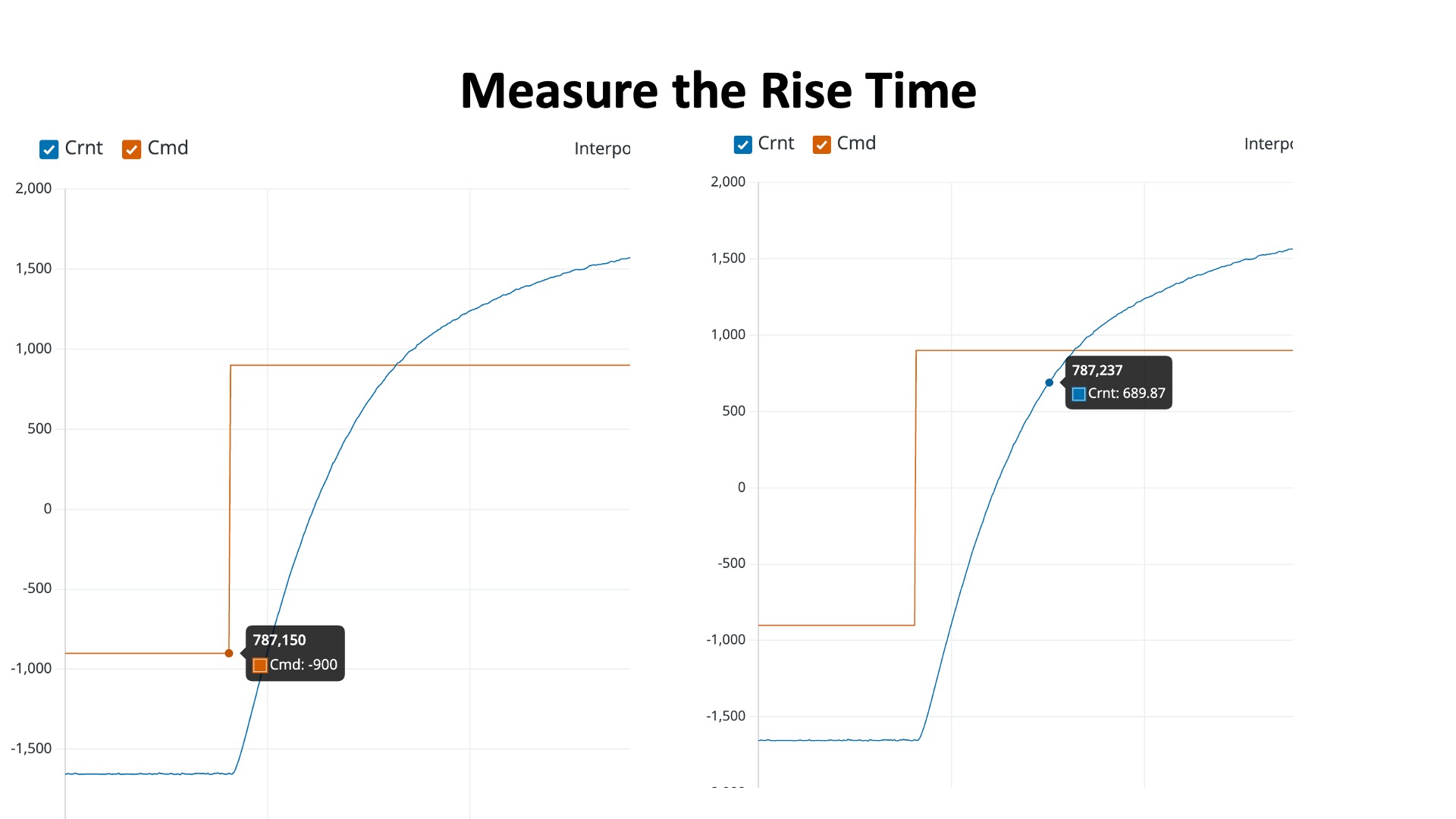
In the three figures below, we show three approaches for estimating \lambda_E:

1. finding the 45 degree phase shift frequency,
2. finding the frequency for which the amplitude is \frac{\sqrt{2}}{2} smaller than at very low frequency,
3. and finding the time to rise by 1-e^{-1}.

If you set the sinusoid frequency to 10, and the input command and the measured coil current are out of phase, like in the picture below, then your current sensor and coil fields are flipped in sign.

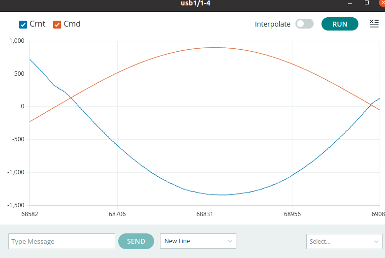
This flipped-in-sign problem is easy to fix. Just change line 206 in the Teensy sketch from

crnt = 10.0*(my6310.adcGetAvg(IN1) - CurrentOffset);

to

crnt = -10.0*(my6310.adcGetAvg(IN1) - CurrentOffset);

If the current trace in mode 0 is flat,  you probably connected the leads to the Hall effect sensor incorrectly. Please check the assembly guide for the correct wiring. The newly revised diagrams under "Add magnetic Field Sensor" are most helpful.

Please be careful to multiple by 2 \pi when converting from frequency in hertz to frequency in radians per second.
NOTICE THAT YOU CAN NOT LEVITATE IN MODE 0 !

4.4) Checkoff One

Once you have found \gamma_{\frac{di}{dc}} and \lambda_E using all three of the above methods (phase, magnitude, and rise time), you are ready for checkoff one.

If your sensor is working properly, and your are using the nonlinear compensation, your SensorScale should be about 0.3 and SensorOffset should be near -2. If yours are far from those values, ask for help.

5) System modeling

The end goal of this lab is to design a stable feedback controller for the maglev system, one whose step response does not overshoot "too much", and is not too noisy. More specifically, you will be designing a lead controller by maximizing a property of the open-loop system's frequency response, its phase margin. You will need a fairly complete CT model of the maglev system to design the lead controller, and to generate that model, you will use a combination of measurements (frequency response as well as step response) and thoughtful analysis.

5.1) Transfer Function Model

Putting together the transfer functions for command-to-current and current-to-position, along with the controller and the feedback loop, we have a complete system diagram, as shown below.

Maglev transfer function block diagram based on linearization (hence all the delta's).

The above block diagram is the transfer-function based model of the linearized Maglev system, including the second-order transfer function relating changes in coil current, \Delta I, to changes in separation distance \Delta Y , and the one-pole model relating changes in Teensy command \Delta C to changes in the electro-magnet coil current \Delta I .

To complete the system model, H(s), we will need to determine values for several parameters, but which parameters are most important for phase margin design? Clearly we can combine the \gamma's for the command-to-current and current-to-separation distance transfer functions, so that we can simplify H(s) to

Since we estimated \lambda_E fromn coil current measurements, there are only two parameters to estimate, \gamma and \gamma_{da/dy}.

You also have a model for the PD controller,

Before beginning this lab, make sure you have finished last week's lab. Then create a matlab model of your feedback system (use the DEFINITELY-NOT-CORRECT values \lambda_E = -1000 , \gamma = 500 , and \gamma_{da/dy} = 2).

Be sure you can use matlab to perform margin plots, compute closed-loop transfer functions, and step responses. Have a quick look at the prelab for matlab hints, and ask if you need help. Also, investigate the impact of \gamma_{da/dy} by increasing its value from 2 to 2000.

From Wednesday's lecture, we used lines of matlab code to test controllers once the variable s has been defined,

s = tf([1,0],1)

and Hs has been specified. We repeat those lines here for the PD controller case and then the lead controller case.

Kp = 5; Kd = 0.1; Ks = Kp+Kd*s; figure(1); hold off; margin(Ks); hold on; margin(Hs); margin(Ks*Hs); figure(2); step(feedback(Ks*Hs,1),1);

K0 = 5.0; sz = -100; sp = -1000; Ks = K0*(sp/sz)*(s-sz)/(s-sp); figure(1); hold off; margin(Ks); hold on; margin(Hs); margin(Ks*Hs); figure(2); step(feedback(Ks*Hs,1),1);

5.2) Determining model parameters.

Finding the model parameters will require a mixture of measurement and insight. Below are some hints to help you get started.

1. Since \gamma_{da/dy} has a limited impact on stability, start by setting it to zero and then determine \gamma by matching the "ringing" frequency of the step response.
2. Once you have determined \gamma, analytically determine the unit step response steady state as a function of \gamma_{da/dy}. Then match the steady-state of the matlab simulation to your measured data.

5.2.1) Determining \gamma

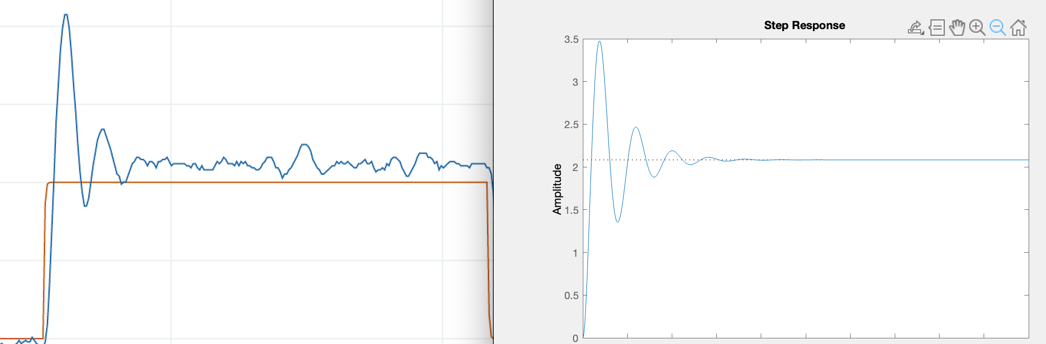
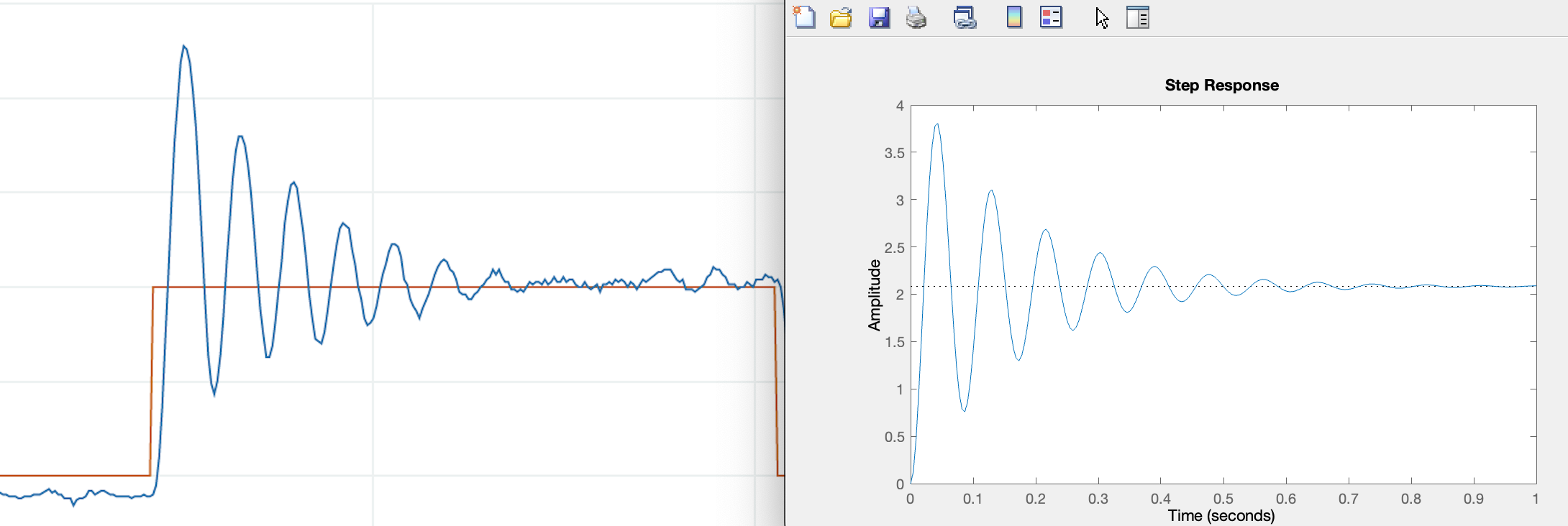
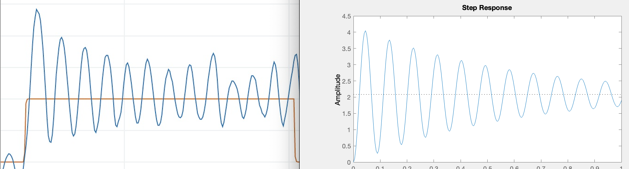
The frequency of the "ringing" in the step response, particularly for the nearly unstable case (like in the third example below), is a particularly sensitive measure of \gamma.

Below we compare PD controller step responses with step responses computed with a well-calibrated matlab model, for K_d = 0.8*K_{d0}, K_d = K_{d0}, K_d = 1.4*K_{d0}, for our optimized K_{d0} and K_p = 5 .

Desired versus measured step responses for a high value of K_d .

Desired versus measured step responses for a middle value of K_d .

Desired versus measured step responses for a low value of K_d .

5.2.2) Determining \gamma_{da/dy}

Desired (red) versus measured (blue) step responses for the PD-control Maglev system. .

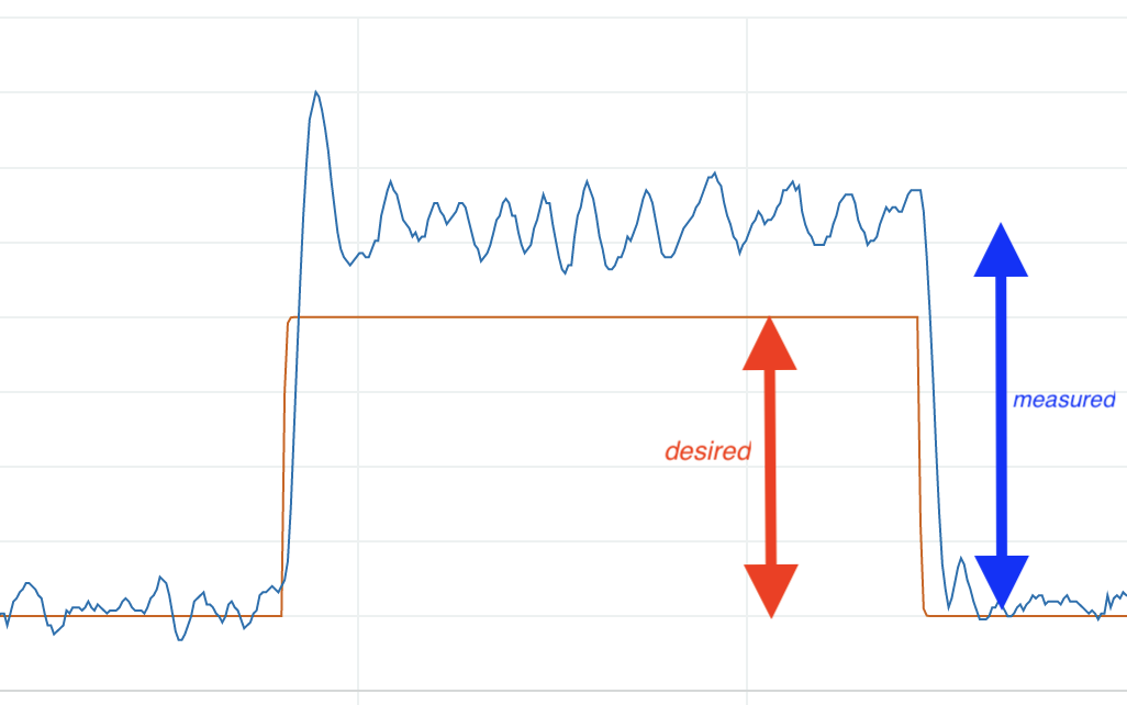
In the figure above, we show annotatation for a plot extracted from the Arduino serial plotter, generated by running the maglev control system with a PD controller. The plot, a comparison of the quasi-steady-state peak-to-peak amplitudes of the desired (red) and measured (blue) umbrella positions, can be used to determine \gamma_{da/dy}. Try determining the formula for the step response steady-state, and then matching.

5.3) Checkoff 2

6) Improved Controller

Now that you have a calibrated model, you can use it to design a lead controller, but then you must also determine how to map your CT lead controller into a DT controller, implement that on the Teensy microcontroller, and test its performance.

6.1) Lead Controller

If we use a PD controller, then

where again K_p and K_d are the to-be-designed proportional and derivative gains respectively. Alternatively, if we are using a lead controller (see compensation ), then where again s_z < 0 , s_p < 0 , and K_0 > 0 are the to-be-designed zero, pole, and steady-state gain of the lead.

6.2) DT Mapping

Our controller determines the Teensy command, c(t), from measurements of the separation distance error, e(t). If we use a PD controller, then

where K_p and K_d are the proportional and derivative gains respectively. But since the Teensy operates on a clock, and only samples y(t) and updates c(t) once every \Delta T, we can approximate the continuous-time controller with a difference equation, where \Delta T is the Teensy update period (0.1 milliseconds for the maglev).

Alternatively, if we are using a lead controller then

where s_z < 0 , s_p < 0 , and K_0 > 0 are the to-be-designed zero, pole, and steady-state gain of the lead. NOTE: recall that you determined a K_p large enough to make your umbrella oscillates, if you use a lead controller, MAKE SURE THE LEAD's K_0 > K_p!!!

6.3) Implementation

Line 217 of the Teensy sketch:

deltaC = 0.0 * pastDeltaC[1] + 0.0 * error + 0.0 * pastError[1];

computes deltaC (which is the MATLAB name for c[n]) from pastDeltaC[1] (which is the MATLAB name for c[n-1], error (which is the MATLAB name for e[n], and pastError[1] (which is the MATLAB name for e[n-1]. To implement the lead controller, you need only replace the three coefficients with values of 0.0 with the values you determined from mapping your CT lead controller to DT.

You could alternatively use the c2d function in MATLAB to calculate the three coefficients.

6.4) Checkoff 3

If we use a PD controller, then

where again K_p and K_d are the to-be-designed proportional and derivative gains respectively. If we are using a lead controller, like in the prelab,

https://introcontrol.mit.edu/fall22/prelabs/prelab07/preLabLead then

where again s_z < 0 , s_p < 0 , and K_0 > 0 are the to-be-designed zero, pole, and steady-state gain of the lead.

Determine a lead controller, implement and test it. We strongly recommend you determine the numerical values for your controller, and then transfer those values to line 217 in the Teensy sketch. Also, we suggest setting the offsetCtype on line 39 to 1 (so that your lead controller is used by default).

Try to keep the high frequency gain, K_0 \frac{s_p}{s_z}, less than 100, so that you do not magnify the measurement noise too much. And match your low frequency gain, K_0, to the value you used for K_p in the PD controller. You may need to lower K_p = K_0 in the PD controller and the lead controller, so that you can make the ratio \frac{s_p}{s_z} large enough to get a good "phase bump" at unity gain frequency.

PLEASE USE NUMERICAL VALUES FOR THE COEFFICIENTS IN THE TEENSY SKETCH!! IT IS FAR EASIER FOR US TO DETERMINE IF THE VALUES ARE IN A REASONABLE RANGE.