Observe and Learn

PLEASE FINISH THE MAGLEV LAB (ADDING INTEGRAL FEEDBACK) before starting this lab.

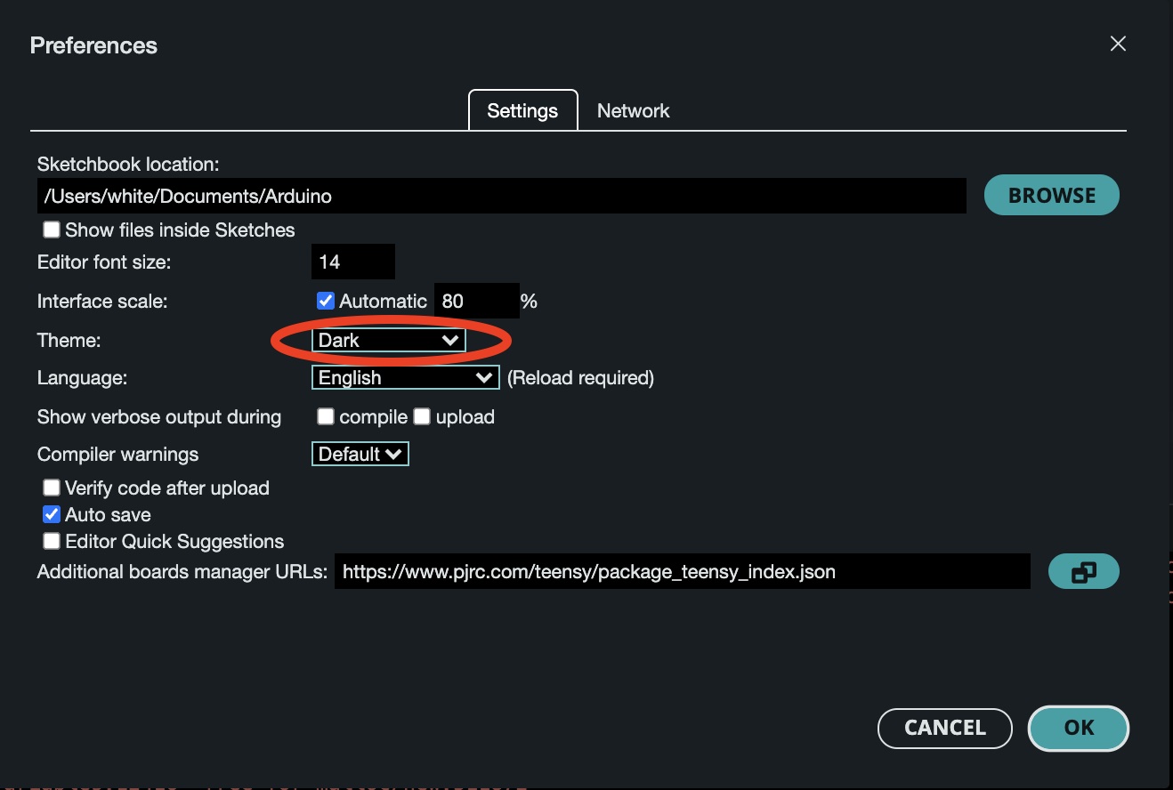
Change to Dark Theme

Makes plots more visible.

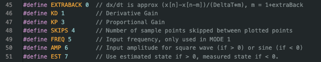
Serial Plotter Send Window Indices

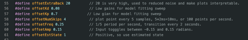
Useful Offsets to Set

Links

• All files for this lab are in one zip is here.
• Please reassemble the two-propeller arm here.
• If you are using the on-line version of matlab, you will need to install the matlab drive connector, available from here.

Task Summary

Week A

1. If using on-line matlab, install matlab connector (linked above).
2. Download the zip file linked above and CAREFULLY follow the software setup directions below.
3. Rebuild double-propeller arm using the assembly guide and this lab's Teensy Sketch.
4. Run a frequency sweeper to measure your rebuilt arm's frequency response.
5. Fit a state-space model to your measured frequency response, and be prepared to explain the results (Checkoff 1).
6. Assess the performance of our default observer-based controller.
7. Compare simulated and measured behavior for tapping disturbances (Checkoff 2).

Week B

1. Optimize your observer-based controller to minimize tracking error and disturbance response(Checkoff 3).
2. Disassemble your kit and return the parts to the bins located in the center of the lab (Checkoff 4).

Introduction

For this lab, you will use a regression-based strategy to "learn" a state-space model directly from frequency response data, and then use this model to design an observer-based state-space controller. Specifically, you will:

1. rebuild the two-propeller arm,
2. run the Teensy sketch in frequency sweeper mode to measure the arm's frequency response,
3. fit a state-space model to the propeller arm frequency response,
4. determine weights for LQR and then use it to compute gains for an observer-based state-space controller,
5. upload your controller to your two-propeller arm, and use your measurements to further optimize the LQR weights.

A few Examples

The above strategy is quite effective, and remarkably robust once the LQR weights are determined thoughtfully, as we show in the three videos below. In each video, the propeller arm is using a controller generated by the above strategy, and is reacting to desired-angle step changes of +/- one hundred degrees. The first video shows the poor performance of the propeller arm with the controller generated by the default LQR weights in the matlab script we provided, the second shows a pretty good controller generated by improving the LQR weights, and the third video shows very similar good performance on an arm with FOUR motors without ANY software changes, just rerunning the sweeper to re-measure the frequency response.

In the leftmost video above, the arm uses the default controller. Notice that the estimated arm velocity, plotted in pink on the computer screen, separates from the measured velocity, plotted in blue, during arm transitions. Note also that the arm overshoots the desired angle significantly, and settles very slowly. In the middle video, the arm uses a controller generated by optimizing the weights. Notice how well the state estimates track the measured states and the limited overshoot. Notice also, the arm's resilience to tapping disturbances. The rightmost video shows an arm with four motors behaving very similarly to the two-motor arm in the second. Exactly the same software that generated the controller for the two-motor arm was used to generate the four-motor arm controller (frequency sweeper, model extractor, LQR weights, etc). That is, the extracted model and controller gains were not the same, but the algorithms to compute them were identical.

Expect to do better

After you've fit your arm with a model, and used the simulation tools to help you determine how to best modify the LQR weights, you should be able to design an observer-based controller that out-performs the pretty-good controller above. In particular, see how close you can get to a rotation step near the sensor limit of +/- 160 degrees. To do that, you will need a controller with far less overshoot than the "pretty good" examples above.

Learning to Model

In all the past labs, we have designed feedback controllers by first developing a model of our system, and then using that model to determine a good controller. As we moved from proportional to PID to Lead-Lag to State-Feedback controllers, we needed progressively more comprehensive models to design these progressively more sophisticated controllers. Unfortunately, our approach to modeling has NOT become more sophisticated. We continue to rely on ad-hoc combinations of physical insight, simplifying assumptions, and measurements.

Until now.

Please follow the instructions below to download and install the software for this lab. When installed correctly, the software allows you to run the Teensy sketch in frequency sweeper mode; capture your arm frequency response in a file (sweeper.csv); fit the frequency response with a state-space model; use the state-space model to to design an observer-based state-space controller; simulate the performance of the controller; upload the controller to the Teensy; and test your controller's performance on your propeller arm. You will also be to change your controller design in matlab, WITHOUT RERUNNING THE SWEEPER, and by rerunning the matlab script and then re-uploading the Teensy sketch, automatically upload the updated controller. The controller will automatically transfer from matlab to the Teensy sketch, no copy and paste required!

Once you have installed the software, please follow the instructions in the assembly guide to reassemble the arm. PLEASE NOTE when calibrating your arm, use the Teensy sketch for THIS lab, 6310_CT_PROP_OBS_SWEEP_SP24, NOT the sketch on the assembly guide page.

Software Setup

The matlab scripts and the Teensy sketch to support this lab are all in one zip file, 6310_CT_PROP_OBS_SWEEP_SP24.zip, linked on the top of this page. Please download the 6310_CT_PROP_OBS_SWEEP_SP24.zip file, but DO NOT UNZIP THE FILE.

If you ARE using on-line matlab, download and install MATLAB Drive Connector, from the link at the top of this page. Matlab drive connector allows you to keep a local sync-ed copy of the files you edit in on-line matlab. Start the matlab drive connector after you have downloaded and installed it, and create a course6310 folder on your local matlab drive.

If you are NOT using on-line matlab, create a course6310 folder in a directory THAT IS LOCAL TO YOUR COMPUTER. DO NOT create the folder in any iCloud directory (MAC), or oneDrive, or Dropbox, or .... These services do not guarantee sufficiently quick file updates, and can interfere with the automatic updating of your controller.

Please move the downloaded zip file to the course6310 directory you just created and, ONLY THEN, unzip the file in the subdirectory. Unzipping the file should create a 6310_CT_PROP_OBS_SWEEP_SP24 subsubdirectory which contains this lab's files: the Teensy sketch, 6310_CT_PROP_OBS_SWEEP_SP24.ino; a main matlab script file, propSS.m, ; five matlab function files; a python program file csvGen23.py, which captures sweeper data into a matlab-readable csv file; and two program-generated files, sweep.csv and obs6310.h. The sweep.csv file is generated by csvGen23.py, and is read by the matlab script. The obs6310.h file is generated by the matlab script, and read when the 6310_CT_PROP_OBS_SWEEP_SP24.ino file is compiled and uploaded to the Teensy.

Click on the propSS.m to open the file in matlab, and click on the 6310_CT_PROP_OBS_SWEEP_SP24.ino sketch to open the file in the Arduino IDE (both files should be in exactly the same directory). If the software is set up correctly, when you run propSS.m in matlab, you should see an update your local version of obs6310.h. Then when you compile and upload the Teensy sketch you opened, it should pick up the sync-ed, updated, obs6310.h file.

Hardware Setup

Please assemble the propeller arm (including the second motor), as shown in the prop linked on the top of the page, but please use the 6310_CT_PROP_OBS_SWEEP_SP24.ino sketch, with MODE set to 0 (on line 15) when calibrating the angle sensor and the motor directions (the AngleOffset is on line 13 and the hbridgeBipolar commands are on lines 367 and 368).

Measuring Frequency Response

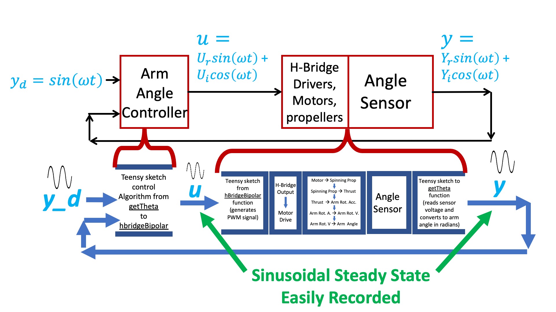
Recall that when we last encountered the propeller arm, we started with a functional diagram of the arm, shown below.

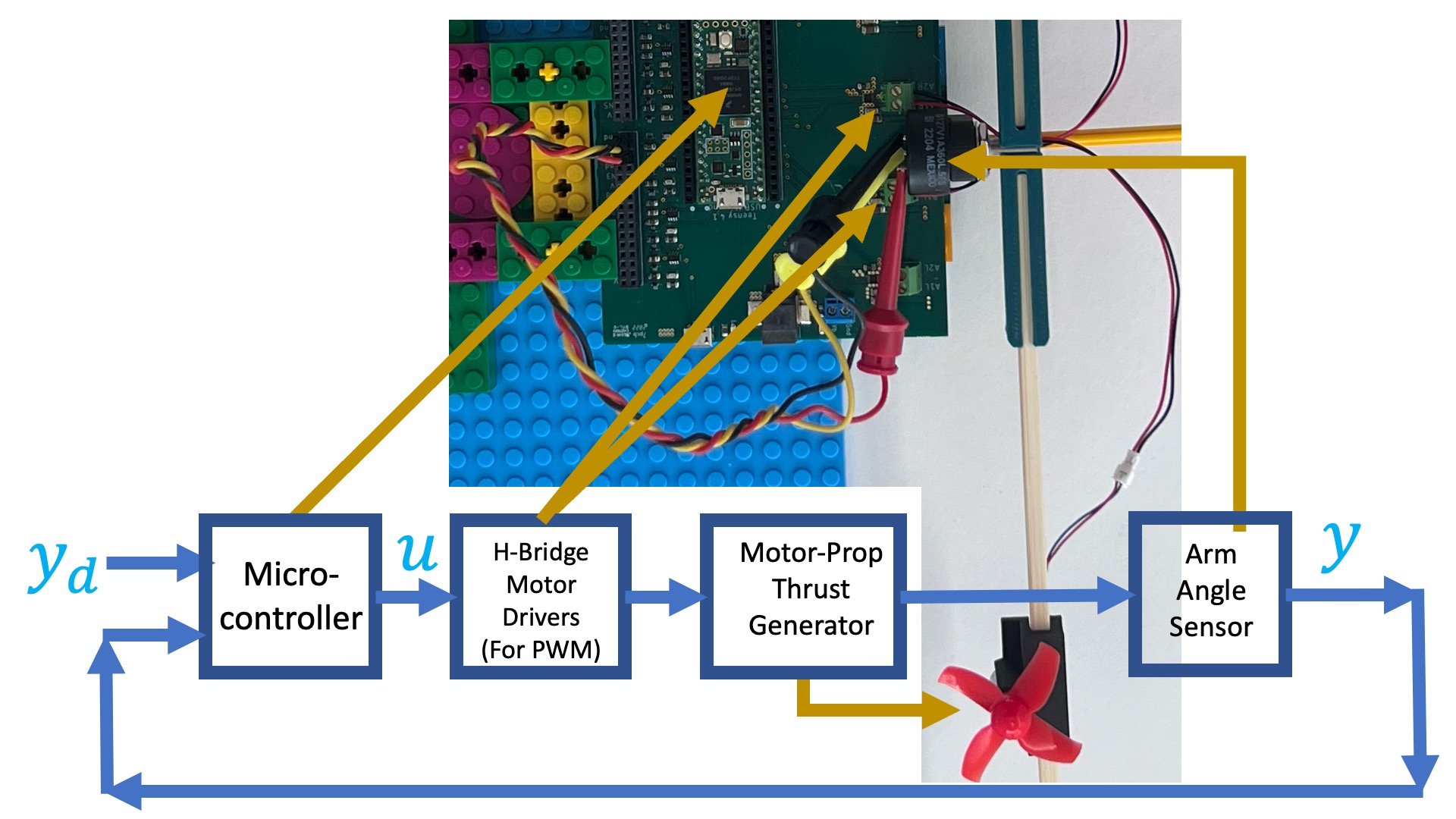
If we are interested in measuring arm frequency response, we can stabilize the arm with a controller. For the stabilized arm, we can set the desired angle to a sinusoid y_d(t) = sin(2\pi ft) = sin(\omega t). If we wait long enough, then the output of the controller, u(t), and the measured arm angle, y(t), will be sinusoids of exactly the same frequency as the desired angle but not exactly the same amplitudes and phases. We can then use the amplitude ratios and phase differences to compute the propeller arm transfer function H(j\omega).

In the control system diagram below, we show the software blocks to clarify the fact that the controller output u is explicitly generated in the Teensy sketch, and that the arm angle, y, is explicitly measured. As a result, we can easily record the magnitudes and phases (or equivalently, real and imaginary amplitudes) of u(t) and y(t).

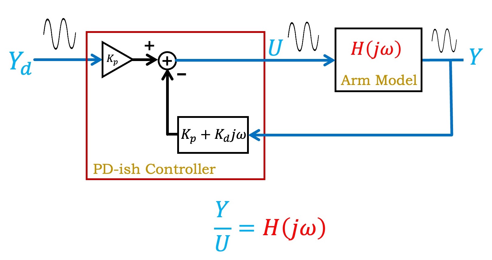
Given the measured sinusoidal steady state amplitudes and phases (or equivalently, real and imaginary parts) for both the command to the arm and the measured arm angle, it is easy to de-embed the arm frequency response from the response of the control system as a whole, as shown below.

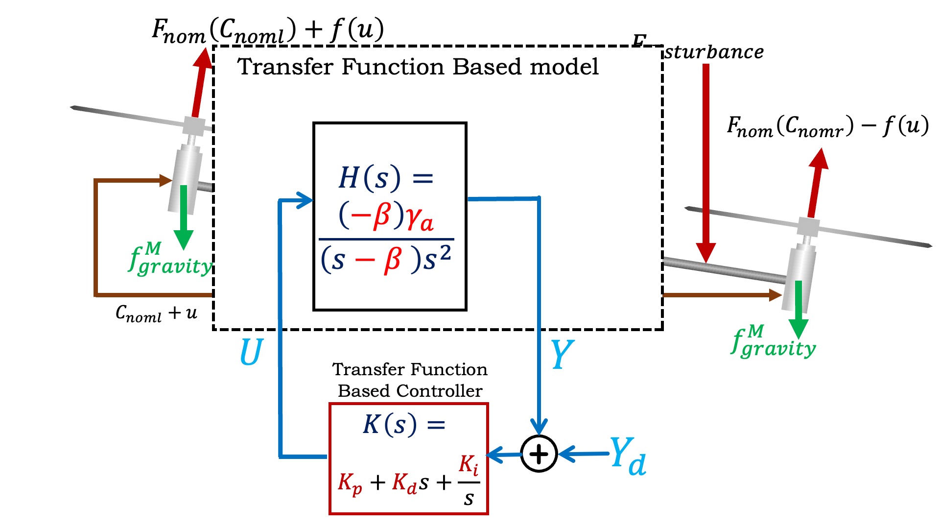
Based on our previous modeling of the arm, we expect that the propeller arm transfer function has three-poles and no zeros. Any three-pole transfer function can be formulated as the inverse of a cubic polynomial,

Do you see why we can represent H(s) = \frac{-\beta \gamma_a}{(s-\beta)s^2)} in the above form? If you compare H(s)'s at s=0, what can you learn about the relationship between a_0, \beta, and \gamma?

Given the sinusoidal steady-state response for a set of frequencies (the sketch we provided measures the response at forty frequencies), and our inverse polynomial form above for H(s), we can set up a system of equations for the a_i's,

Cross-multiplying and reorganizing yields a set of linear equations for the a_i's,

You will be using a matlab fitter that approximates H(s) by solving the above set of equations (using a variant of least-squares), and then converts the transfer function to a state-space model. As we noted in the last lab, transfer functions do not uniquely define state-space representations. You will have to examine the state-space matrices generated by the matlab fitter to determine how it assigned the states.

Running the sweeper

After you have calibrated your arm, please set the MODE on line 15 in the Teensy sketch to -1, make sure both power supplies and your laptop are connected to the controller board, and then

1. Open a terminal or powershell window in the 6310_CT_PROP_OBS_SWEEP_SP24 subdirectory, and try typing "python csvGen23.py" (or python3 if you have both python2 and python3 installed) in that window. If you do not get an error in a couple of seconds, type control-C in the window to stop the program.
2. If you got an error like "serial.tools....not found..", type "python -m pip install pyserial" followed by return in the command window. If you get an error associated with matplotlib, type "python -m pip install matplotlib". If you are using python3, type the above commands, but substitute python3 for python.
3. Upload the sketch (with MODE set to -1) onto the Teensy, close the serial plotter if it is open, and then open the serial MONITOR by clicking the circular icon at rightmost top of the arduino IDE window.
4. You should see you arm oscillating and after about twenty seconds, you should see a set of numbers in the arduino monitor window.
5. CLOSE THE SERIAL MONITOR WINDOW.
6. Type "python csvGen23.py" or "python3 csvGen23.py" followed by return in the terminal window, and you should see numbers start to appear (like in the video below). It can take ten seconds or more for the first numbers to appear.
7. Let the sweeper run through its forty frequency points at least twice (should take less than 10 minutes). Then type control-C to stop the python program.
8. Sometimes the above strategy fails, and the python program never prints any numbers. Be sure that the serial plotter is NOT OPEN, then try, WITHOUT QUITTING THE PYTHON PROGRAM, reopening the Teensy serial monitor, waiting until numbers are printed, then reclose the serial monitor. That may be enough for the Arduino to "release" the USB receiver so that the python program can connect. If that does not work, quit everything (Arduino, Teensy and python), and try again.
9. Run the propSS matlab file in matlab, it should pick up the recorded frequency response and create a model.

The video below shows the sweeper sweeping (using a PREVIOUS TERM's setup!).

After matlab fits the model, you should be able to type the matrices A, B, and C in the matlab command window, and see reasonable values.

Checkoff 1

Please rebuilt your arm, run the sweeper, collect the sweep data as described above, and generate the state-space model.

Observer Estimate

For the maglev system, we could directly measure the states of the system, thanks to a combination of the optical distance and the hall-effect field sensors. For the propeller arm, this is not the case. Differencing angle sensor readings is a noisy way to estimate arm velocity, and measuring propeller thrust is even more problematic. Instead, since we used a frequency sweeper and fitter to generate an accurate model for the arm, we will use simulation of that model, with angle measurement corrections, to estimate the equivalent of the arm's velocity and the net thrust.

Using a state-space controller and an observer-based state estimator requires two sets of gains, controller gains (the K's), and estimator correction gains (the L's), and we will need insight into how to select those gains. Below we remind you of the transfer-function based model of the arm, and in a step-by-step fashion, substitute in a state-space model and then an observer, underlining the insights helpful for picking gains along the way.

TF Modeling and PID Control Review

To transition from transfer function to state space modeling and control, consider the "schematic" diagram of the arm and controller, shown below.

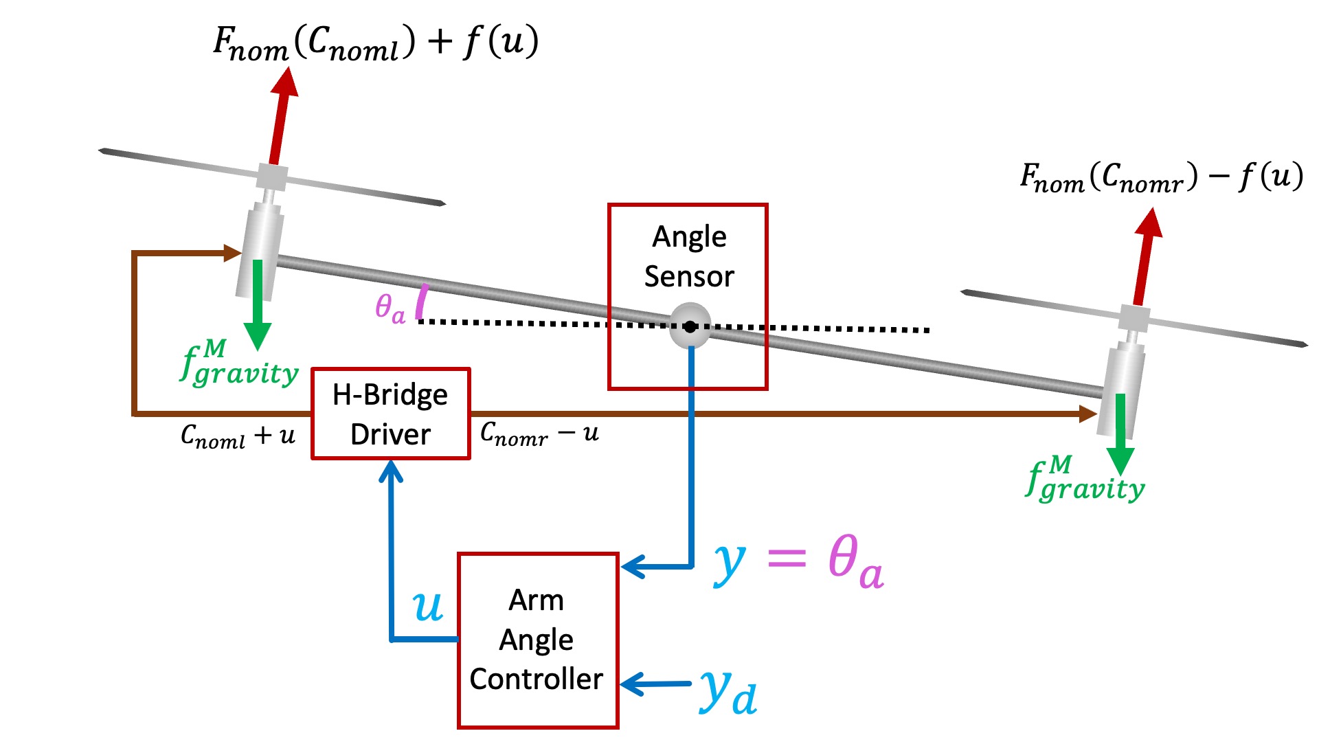
We used physical insight to uncover a transfer function description of the propeller arm, used measurements to calibrate the model, and examined pole locations and disturbance transfer functions to determine good PID controller gains.

State-space and Observer-based Control

We can replace the transfer function model of the arm with a state-space model, as shown in the figure below. Also shown in the figure is the PD-ish controller that was used to stabilize the arm, which made it possible to measure the unstable arm's frequency response.

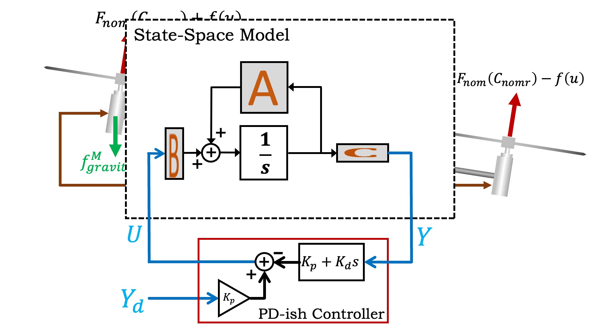
Since you synthesized a state-space model from frequency response measurements of your particular arm, you can expect that your model is accurate. And given an accurate state-space model for the arm, you can use it to generate an observer. The observer time-evolves a simulation of the state-space model, with corrections based on comparing predicted and measured outputs (angles in this case). These continuously-corrected estimated states are then used for estimated-state feedback, as show below.

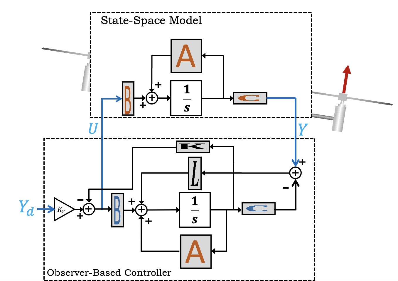
As the above figure makes clear, when we use an observer-based state-feedback controller, we have two sets of gains to determine. The first are the state-feedback gains (the K's), and in the last lab, you learned how use LQR to determine those gains. The second set of gains are the observer, or state-correction, gains, which can also be determined using LQR.

When using LQR to determine state-feedback gains, one sets relative state weights (Q) by determining which states should go to zero fastest, and the relative control weight (R) based on ensuring the commands do not become too large. When using LQR to determine observer gains, the intuition to apply is less obvious.

In class we learned that the poles of the control system are eigenvalues of A-BK, and poles of the estimation error system are the eigenvalues of A-LC, so we can compare the two sets of poles to see if the estimation error is converging much more slowly than the controller. But what is too slow? And for systems with multiple poles, how should we compare? And how should we modify the LQR weights if we decide the estimator is converging too slowly?

As we will see later in this lab, we can also investigate measured and simulated responses to typical disturbances, to help us decide which observer errors should go to zero fastest, and therefore be assigned the highest LQR weights.

Checkoff 2: Examining the Default Controller

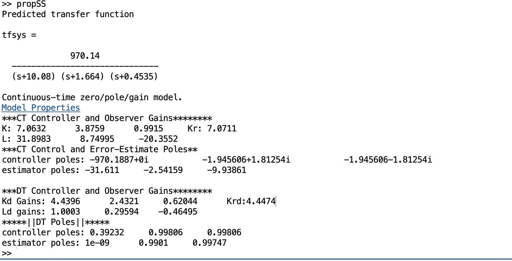
Run the propSS.m script in matlab, enlarge the command window and spread out the four plots it generates, so you can see all the results. In the command window, as shown below, you can see a transfer function representation of your state-space model and can determine the model's poles. You can also see the gains and the associated controller and estimator poles for the CT and DT controller (note the Teensy uses the DT controller). Your poles and gains will not match these, because your extracted model is different.

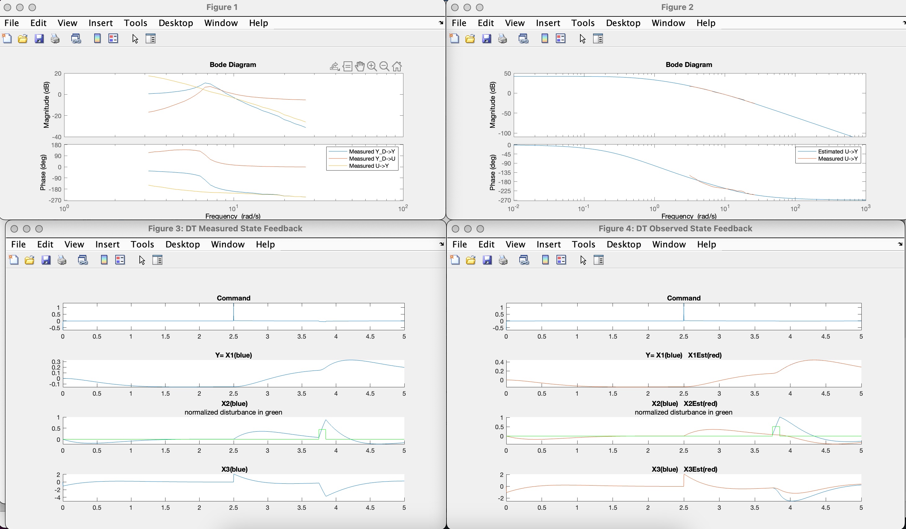
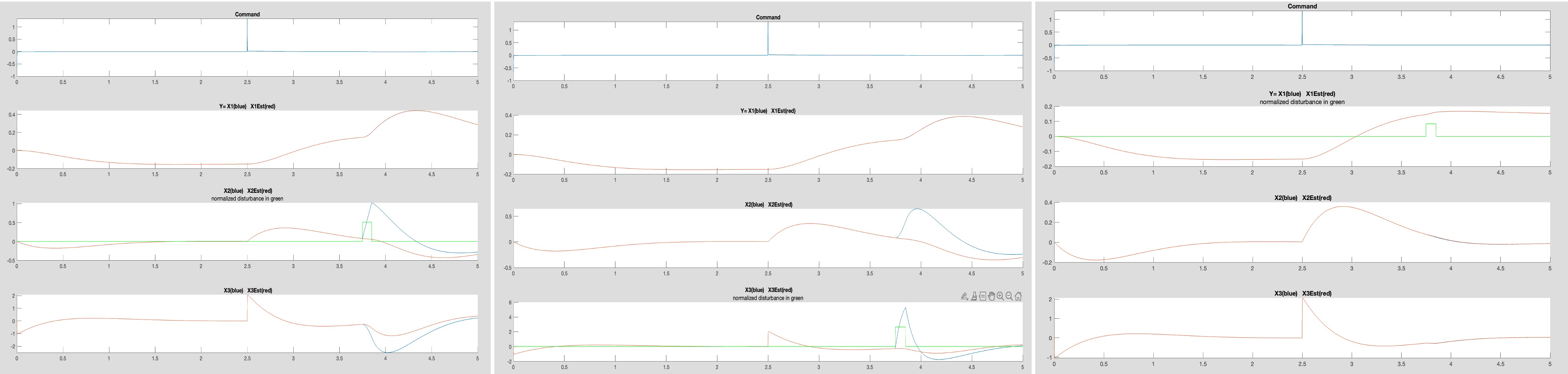
Your plots should be similar to the ones below (though note again, your model will be different from ours, so your plots will NOT be identical). You should be able to see two fitting results (top two plots in the figure below), and two simulation results (bottom two plots in the figure below). Examine the two simulation plots, what can you learn about the default observer-based controller? Is it fast? Does it recover from disturbances quickly?

Try rerunning propSS.m with the disturbance acting on equations 1, 2, and 3 (change disturbEqn on line 31 of propSS.m), you should be able to see results like the ones below (from left to right, the plots show the disturbance in equation 2, 3, and then 1). Again, yours will be different because your extracted model will be different.

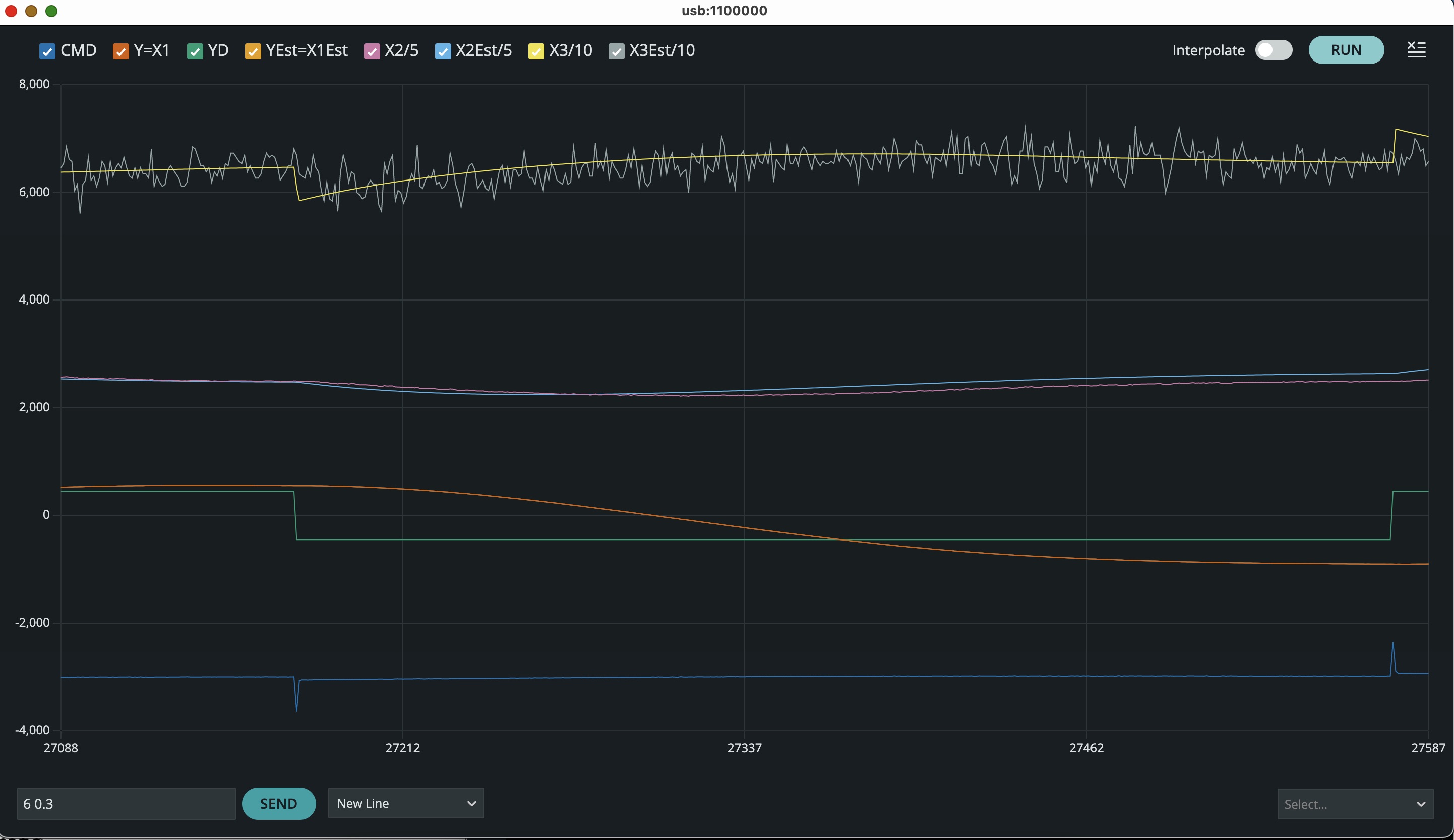
Set the MODE to 1 in the Teensy sketch (control w/observer), be sure you first run the propSS.m script in matlab to generate the include file for the sketch, and then upload the Teensy sketch to the Teensy (make sure both power supplies and your laptop are connected). Type "6 0.3" in the plotter send window, to increase the step size, and you should observe a plot like the one below

What can you learn about the default controller? Is the state estimation effective? Is the control?

Now try "tapping" the arm with a pencil or a chopstick. You should observe responses like the figure below when you "tap" the arm.

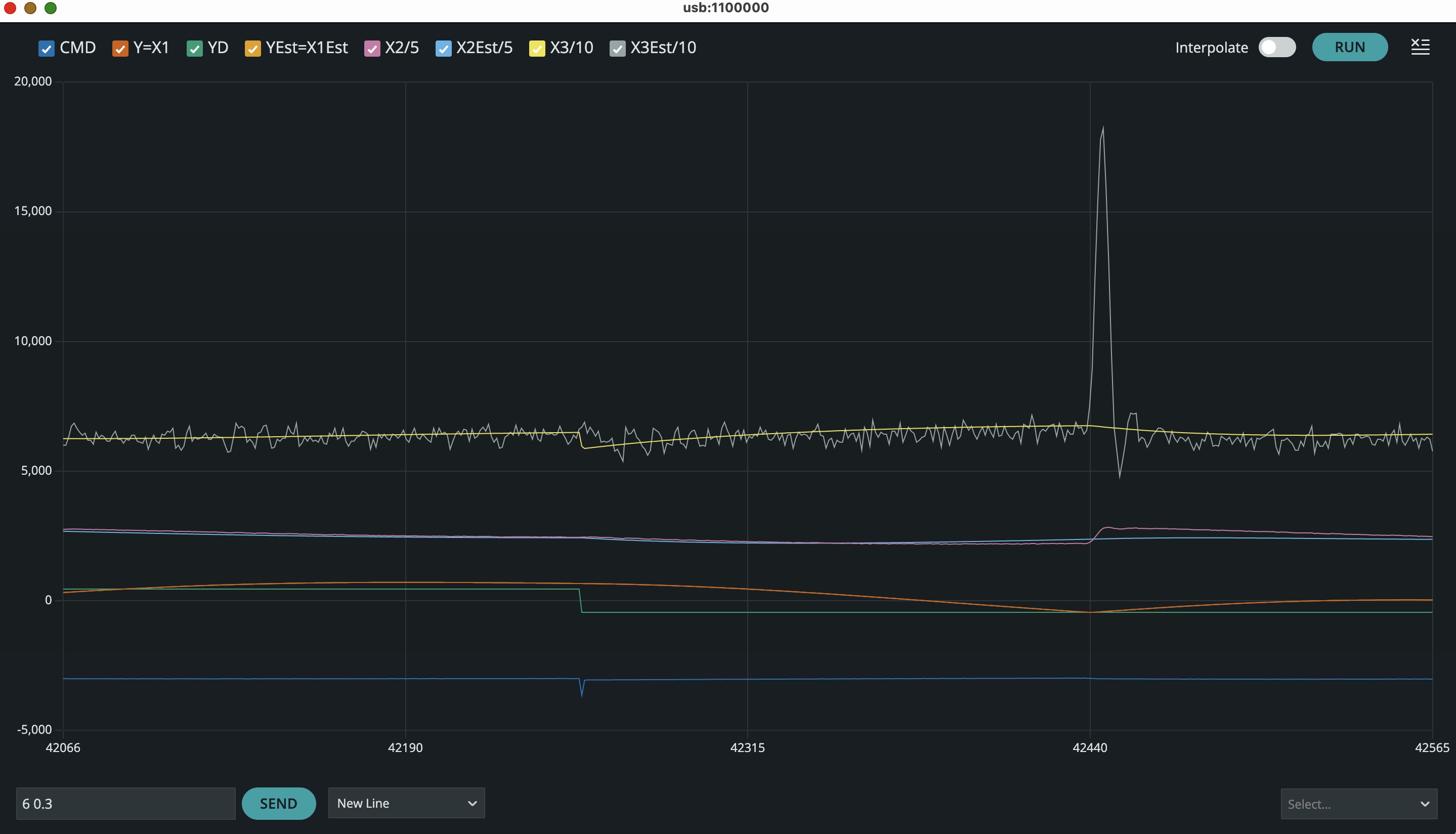
Examine the three simulation plots with disturbance acting on equations 1, 2, and 3. Which simulation mostly closely corresponds to what you see when you tap your propeller arm (note that the in the Teensy plotter, the X3 state is at the top, but in the matlab simulation plot, the X3 state is at the bottom)? Since tapping is a typical disturbance, what do your simulation and experimental results tell you about the state estimation errors? That is, which state's estimation error should be driven to zero fastest, and what does that tell you abou the observer LQR weights (Ql and Rl in the matlab propSS.m file).

STOP HERE FOR WEEK A!

Checkoff 3: Mind your K's and L's.

Use what you've learned above and adjust the LQR weights for both the controller and the observer in propSS.m (lines 51 \rightarrow 53 and 60 \rightarrow 63), and then test your controller on the arm using smaller step-sizes, +/- thirty degrees or less. Try to minimize the command noise without compromising performance.

Notice also that the discrete-time L_d's, computed on line 122 of propSS.m, use scaled values of the continuous-time Ql and Rl matrices set on lines 60->63. Alternatively, you could use the place command to compute the L_d's, as we show (commented out) on line 123. Note that the commented-out place command has an error (it is missing a transpose), and the pole locations specified are probably far from optimal.

You can simulate the interaction between L_d gains and controller command noise (very approximately) by removing the 0.0 from line 27 of propSS.m. Examining the noise simulation may help you design better observer gains.

A Fitting End with a Nagging Question.

After you complete this lab, you might think that the fitting approach works so well, and seems so automatic, that maybe you did not need all of the material we covered in 6.310. If you are having such second thoughts, please think about using the approach for a completely new problem.

You'll have to decide what to actuate and what to sense. And since you can only measure frequency response if your system is stable and nearly linear, you will have to decide how to linearize and stabilize your system. And if you stabilize your system with a classical controller, you will have to determine how to de-embed the controller from the measured frequency response. How many frequencies should you measure, and over what range? And how will you "regularize" the regression? And once you generate the model, how do you determine the LQR weights for the controller and the estimator? What experiments will you try?

Oh and one last nagging question. Consider the relationship between \hat{y_f}, the feedback contribution to the controller output u, and the y's, the entire past history of measured angles. Abstractly, the observer-based controller is summarizing all the past measurements with a few internal states, and is then updating u with a weighted combination of those states. Maybe we could pick better states? Or fewer states? Maybe we could determine (or learn) better ways to update the state, and better weights to use when determining u? Statistical estimation, model-predictive control (MPC), H_{\infty} control, and reenforcement learning (RL), are a few of the many control topics that touch on these issues, ones we did have time to cover this past term.

There is much more to the control story, and of course, many more classes to take.

Congratulations! You have completed 6.310/2!!