Sequences and Difference Equations

The questions below are due on Thursday February 15, 2024; 10:30:00 PM.
 

1) A Crane Example

A heavy cargo crane travels on a track above a buried beacon, as shown in Figure 1. The crane measures its signed distance to a beacon \Delta T times a second, where by signed distance, we mean that the distance is negative if the crane is to the left of the beacon and the distance is positive if the crane is to the right of beacon (as shown in figure). The crane can move itself along the track and thereby reposition itself in response to a change in the desired position.

Crane traveling on a track and measuring distance to a Beacon.

The most common way to vary the motion of a vehicle is to increase or reduce its energy supply, either in the form of fuel or electric current, resulting in an increase in vehicle acceleration or deceleration. For example, you can increase the copter motor's electric current or depress the gas pedal to increase a car engine's fuel supply to increase the acceleration. It is also common for motors to include an internal controller that adjusts acceleration to maintain a desired velocity. For example, we adjust current to control acceleration for the small copter motor we use in this course (referred to as a brushed motor), but the professional quadcopters use larger brushless motors that always include velocity control electronics.

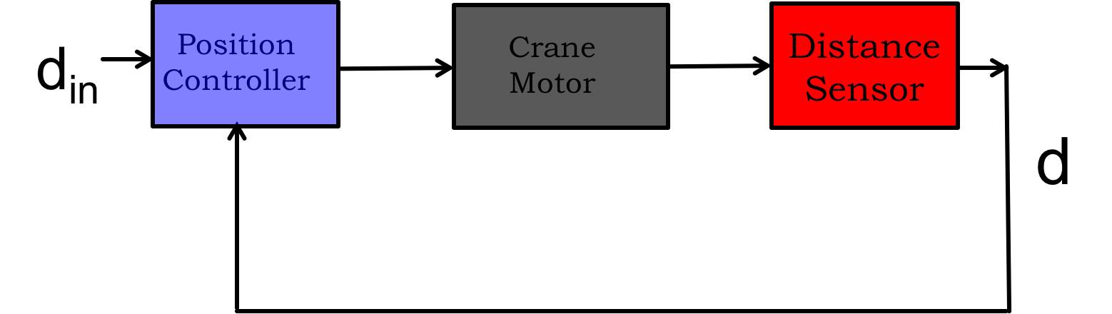
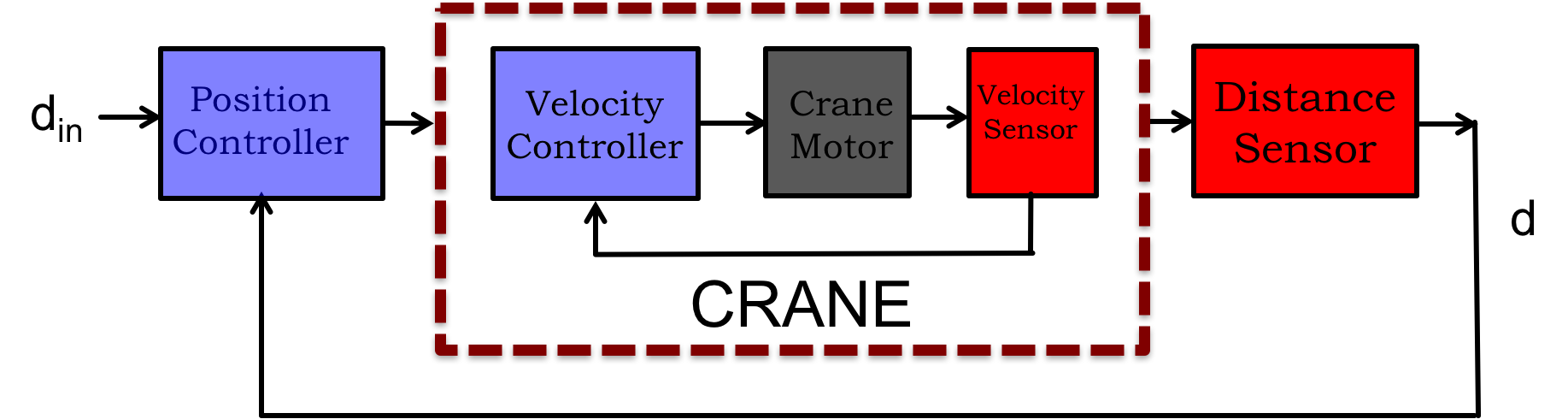
If our job is to design a position controller for the crane, then the output of our controller might directly adjust the acceleration of the crane motor, in which case our feedback system would be described by the block diagram in the first figure below. Or there might be a velocity controller inside the crane, in which case our controller will adjust crane velocity, and our feedback system would be described by the diagram in the second figure below. And since we will use a microcontroller to implement our design, we will have to determine how often to sample the crane position and update the our acceleration or velocity commands.

Crane direct proportional controller.

Crane proportional controller with internal velocity controller.

Are different controllers needed for the two different situations? How long will it take to get the crane to the right position? If we try to position the crane too fast, will it overshoot and have to backtrack? How often should we sample and update, once a minute, once a second, once a microsecond? We will need models to help us answer these questions, but what kind of models?

Since we are using a microcontroller that can be programmed to sample a sensor and update an actuator at a fixed rate, we need a modeling strategy that can inform us about how the sequences of sensor samples and actuator updates evolve. As we will see in the remainder of this section, models based on difference equations are particularly suitable.

2) The Discrete Mindset

We experience a world that evolves in continuous time, full of physical objects whose trajectories are accurately modeled with differential equations. We drop a ball and gravity accelerates it. The ball's acceleration is the time derivative of its velocity, and its velocity is the time derivative of its position. But from the perspective of a computer, the continuous-time world must be reconstructed from a series of samples collected at discrete time-points. A computer only sees the world in discrete "samples" and a falling ball's velocity must be approximated from differences in successive position samples, its acceleration approximated from the change in position differences from one pair of samples to the next.

One might wonder if the computer's discrete-time perspective is more accurate. Perhaps continuous time is just a convenient model for what is actually discrete, just as Newtonian mechanics is a convenient model for what is actually quantized. But such musings are best left to scientists and philosophers. As engineers, we have work to do. Computers, in their many forms (digital signal processors, microprocessors, micro-controllers, etc), are powerful tools that are pervasive in engineering design. We can work with them more effectively if we understand their perspective.

On the computer, it is more natural to think in terms of sequences. Derivatives in time become differences between samples, integrals become sums, and physical system trajectories governed by differential equations become sequences governed by difference equations. Adopting this perspective from the beginning can help us design better systems. And as an added benefit, you can study this subject even if you have not yet studied calculus or differential equations.

In this section, we will use a number of examples to introduce:

1. Our notation for sequences and linear difference equations (LDEs),
2. How to model a physical problem using LDEs,
3. How to solve first-order LDEs by computing *natural frequencies*,

This class focuses on control problems that can be modeled with linear difference equations (LDE's), a surprisingly rich topic both theoretically and practically. And in this first section, we study homogenous LDE's, that is, LDE's with initial conditions but no inputs. We chose homogenous LDEs so that we can emphasize three central concepts:

• LDE's and the systems they represent have *natural frequencies*
• If an LDE has a natural frequency with magnitude greater than one, the generated sequences will grow exponentially. We say such LDE's are unstable.
• If a first-order LDE has a negative natural frequency, the generated sequences will oscillate. If the magnitude of a natural frequency is less than one, the LDE is stable and the oscillations decay to zero eventually. Otherwise, the LDE is unstable and the oscillations will grow.

3) Sequences

For us, sequences can be considered to be a set of values indexed by an integer. Such sequences are useful for representing discrete-time data in a variety of applications, including digital audio, stock prices, bank balances, and control applications. For example, the Arduino-based controller for your copter-levitated arm has three sequences: two sequences of samples (the analog inputs from the propellor-motor and angle-sensor) and a sequence of outputs (the analog output to the motor driver transistor).

We will use, and translate between, three representations for sequences: explicit enumeration, closed-form expression, and implicit definition using difference equations and initial conditions. (Difference equations are a special case of the recurrances commonly studied in discrete mathematics.) As an example, let y be the sequence of powers of \frac{1}{2}. The sequence can be represented by explicit enumeration

or by closed-form expression,

or with a difference equation and an initial condition,

We've opted for a standard notation to represent sequence values, though it's worth mentioning that this choice isn't universally adopted. Throughout this course, we'll consistently use brackets to indicate the indices for sequence values.

In some cases, it can be clearer to graph short explicitly-enumerated sequences using “lollypop" or stem plots. For example, below is a stem plot (created using MATLAB) for 200 samples of a sequence generated by roughly twenty milliseconds of a sound sampled eight thousand times a second.

Stem plot of 200 samples of a sound (roughly 20 milliseconds)

As must be obvious from the plot, stem plots can be cumbersome for long explicitly-enumerated sequences. For longer sequences, it is common to use the standard connect-the-dot plots, even though there is no meaning to the values between sequence entries. Connect-the-dots plots are used, for example, in our software for plotting real-time results from the copter-levitated arm.

4) Linear Difference Equations

As noted above, sequences can be represented implicitly, where an equation is given that relates one element of a sequence to other elements. For example, the elements of a power sequence satisfy

Implicit representations of the above form are referred to as homogenous first-order linear difference equations (LDEs): difference equation because we are computing differences between sequence values, linear because we are using linearly scaled sequence values, first-order because only one difference is being computed, and homogenous because the difference equation is equivalent to insisting that a particular weighted combination of adjacent sequence values must sum to zero (as shown above).

Note that a first-order LDE does not completely specify a sequence, one must also specify the value of y[n] for one value of n. If one specifies y[0], as is most common, then y[0] is referred to as an initial condition for the first-order LDE.

As an example, if y[0] = 5 and \lambda = \frac{1}{2} then the solution to the homogenous first-order LDE is

but if y[0] = 3, then the solution to the same LDE is

Another well-know sequence with a homogenous LDE representation is the Fibonacci sequence, in which the next element in the sequence is the sum of the previous two. That is,

The LDE for the Fibonacci sequence has two differences, so we refer to its associated LDE as second-order. And to completely specify the sequence generated by a second-order LDE, it is necessary to provide two initial values. To generate the classical Fibonacci numbers, set y[0] = 0 and y[1] = 1. Then, using the LDE, it is easy to explicitly enumerate the rest of the sequence values,

In general, an LDE, together with initial conditions, defines an infinite sequence of values, y[0], y[1], y[2], \ldots. We say an LDE is kth order when y[n] depends only on the k previous values of the sequence y. That is, a kth order homogenous LDE has the general form

where a_1, \ldots , a _ k are LDE-specific constants.

The above LDE is referred to as homogenous because we can rewrite the equation as

The above rewrite means an LDE can be interpreted as requiring that a particular weighted combination of adjacent sequence values sum to zero. Therefore the sequence of all zeros will always satisfy the LDE (but not necessarily the initial conditions). Or said another way, homogeneity means that if y[n-1], y[n-2], \dots y[n-k] are zero, then so is y[n]. When we add inputs, later, they will replace the zero on the right side of the rewritten homogenous LDE.

As we will see below, it is easy to solve and reason about systems described by LDEs. So even though most systems are not precisely linear, we often model them with LDEs even if the model is not an exact fit. An easily analyzed, but imperfect, LDE model is likely to be more helpful in design than an accurate non-linear model that is nearly impossible to analyze.

5) The Natural Frequency in First Order LDEs

The simplest LDE is the homogenous *first order* LDE, whose form we have already seen,

We already know that we must specify an initial condition, y[0], for the solution of the LDE to be unique.

There are many ways to calculate the values of a difference equation, so if we wanted to know y[n], we could compute it relatively easily by starting with the initial conditions, and propagating forward. Such a method is referred to as “plug and chug", and as the name suggests, is more perspiration than inspiration. In particular, plug-and-chug offers little insight into the sequence's general behavior.

Instead, we can derive a closed form for y, one that provides insight into the general behavior of the sequence. In the first-order case, we can derive a general form almost by inspection. To start, we expand the LDE as in

Question:How does a computer calculate \lambda^ n, and is it faster than n multiplications by \lambda ?

The above derivation yields a direct formula for y[n] as a function of y[0] and \lambda, a formula that can be evaluted far more efficiently than plug and chug, particularly when n is large. But the derivation also reveals a more general idea, that changing the initial condition only scales the associated sequence, but changing \lambda alters how the sequence evolves. For this reason, we refer to \lambda in the first-order LDE as its natural frequency.

As we will see in the examples that follow, the natural frequency of a first-order LDE, or equivalently \lambda, governs the evolution of its associated sequences. In particular,

• If \lambda \gt 1 , the sequence grows monotonically and without bound, and we say that the first-order LDE is *unstable*.
• If 0 \lt \lambda \lt 1 , the sequence decreases monotonically to zero, and we say that the first-order LDE is *stable*.

What if the natural frequency of a first-order LDE is negative? To answer that question mathematically, consider two first-order LDE's,

These two first-order LDE's have negative natural frequencies, -\frac{4}{3} and -\frac{3}{4}, respectively.

Before moving on, take out pencil and paper and sketch out the stem plots for the sequences y_a and y_b assuming initial conditions y_a[0]=1 and y_b[0]=1. (Hint: You can use plug-and-chug to determine the values of the sequence.) Compare and contrast the sequences.

5.1) Banking (An Interest-ing Example)

Suppose you put $100 into a high-interest bank account 30 years ago and forgot about it. The account paid 12% interest per year, how much do you have now?

If we assume that the interest was compounded annually (meaning the interest is added to your account balance once a year), we can represent your bank balance as a sequence, y, where y[n] is your bank balance n years after you opened the account. Then y[n] can be related to y[n-1] by adding the 12 % interest, leading to a first-order LDE,

The initial condition for the LDE is the initial bank deposit, so y[0] = 100.

The bank balance LDE has a natural frequency of 1.12, so we know that y[30] = 100 \cdot 1.12 ^{30} \approx $3000. Not bad. But what if one of your parents had opened the account for you 60 years ago? Then you would have y[60] = 100 \cdot 1.12^{60} \approx $90,000! Such exponential growth is expected whenever an LDE has a natural frequency greater than one. Although in this case, the natural frequency is 1.12, and is not that much larger than one, so the exponential growth is not that fast.

5.2) Interest not in your favor

Suppose you put $100 into a checking account 30 years ago and forgot about it. If the bank charges checking accounts a 5% fee, and deducts it annually, how much is still in the account?

The checking account can also be modeled as a first-order LDE, just like before, but with funds removed rather than added,

The natural frequency of this LDE is 0.95, and we can use it to determine the amount left after 30 years, y[30] = 100 \cdot 0.95 ^{30} \approx 21. Not much.

Now, forget about that checking account fee from above. Suppose you're collecting interest in the bank and it pays at 12 % per year, but it compounds that interest monthly. We can rephrase this to say suppose 1 % interest was added to your account every month. Then how much would you have after 30 years and after 60 years if you started with $100?

Consider the following questions before moving on:

• What if the bank paid 12 % interest per year, but compounded interest daily, so that \frac{12}{365} % in interest was added to your account every day? How would your balance change after 30 and 60 years?
• And what if the bank compound interest hourly? How would your balance change after 30 and 60 years?

6) More First Order LDE Questions

For the problems below, consider the sequence y[n] defined by the difference equation:

If y[10] = 3 and y[11]=2, determine \lambda and y[0]:

7) Summary

A first-order homogenous LDE has the form

and given an initial condition, y[0] , the solution to the LDE is given by We refer to \lambda as the natural frequency for the difference equation, and for the first-order LDE, and ONLY for the first-order LDE, the natural frequency is equal to the LDE coefficient. For higher-order LDEs, this will not be the case.

From the two bank balance examples, we saw that the natural frequency of a first-order LDE, or equivalently \lambda, governs the evolution of its associated sequences. In particular,

• If \lambda \gt 1 , the sequence grows monotonically and without bound, and we say that the first-order LDE is *unstable*.
• If 0 \lt \lambda \lt 1, the sequence decreases monotonically to zero, and we say that the first-order LDE is *stable*.
• If \lambda = 1, then the sequence does not change value with index, and the first-order LDE is neither *stable* nor *unstable*.

When the natural frequency is negative, the associated sequence values oscillate between negative and positive. In addition, when the magnitude of the natural frequency is greater than one, the associated sequence values grow in magnitude, and when the magnitude of the natural frequency is less than one, the sequence values decay to zero. In particular,

• If \lambda \lt -1 , the associated sequences oscillate, the magnitude of their values grow without bound, and the first-order LDE is unstable,
• If -1 \lt \lambda \lt 0, the associated sequences oscillate, their values decay to zero, and the first-order LDE is stable,
• If \lambda = -1, the associated sequences oscillate, the magnitude of their values neither decay nor grow, and the first-order LDE is neither stable or unstable.