Crane Control and Root Loci

The questions below are due on Thursday February 29, 2024; 10:30:00 PM.
 

1) First Order Crane Example

Crane traveling on a track and measuring distance to a Beacon.

Crane proportional controller.

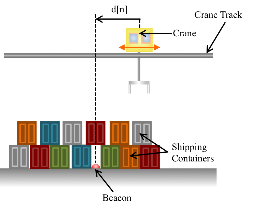
Recall that the distance from the beacon for the velocity-controlled crane, in Figure 1, is described by the difference equation

where d[n] and v[n] are the n^{th} measured distance and controlled velocity respectively. Recall also that if we use the controller as diagrammed in Figure 2 with proportional feedback, then the velocity is given by where K_p is the proportional gain and d_{in} is the input, or desired, position. And finally, recall that the behavior of crane and controller can be described by to arrive at a first-order LDE with an input, d_{in}.

The single natural frequency for the above first-order LDE for d[n] is a simple function of proportional feedback gain, and is given by

When determining gains for a control system, a plot of how the natural frequencies change with feedback gain is often easier to generate than an explicit functional form, and often lends more insight. We show such a plot of natural frequency versus gain in the figure below.

The points in the plot below are the natural frequencies for different gains for the above system. Note that the plot shows the natural frequencies as points in the complex plane (x-axis for real, y-axis for imaginary), even though they are real for first-order systems. This is because, as we have already seen for the case of second-order systems, natural frequencies are the roots of a system-specific polynomials, and in general are complex. Also, we refer to the plots like Figure 3 as a root-locus plots, because the curves in the plots are formed from the "locus" of roots of the polynomials generated by sweeping a system's feedback gain from zero to infinity. Finally, root-locus plots for discrete-time systems often explicitly denote the unit circle |\lambda| = 1, because a system with a natural frequency outside the unit circle is unstable.

Root Locus For Crane with Velocity control.

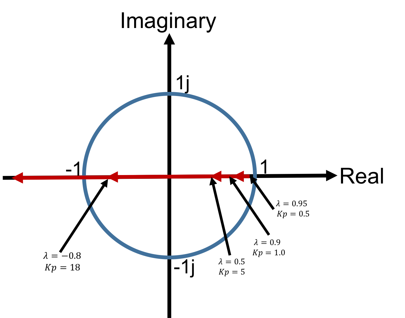
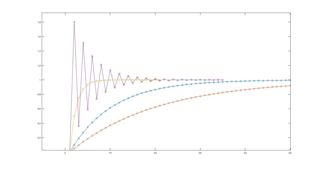
The arrows in the red curve of Figure 3 show the path of the natural frequency with increasing gain. As the plot shows, with increasing gain, the natural frequency moves from close to one, towards zero, then towards negative one, and finally outside the unit circle. The step responses for the system, in Figure 4, show the same trend with increasing gain. As the gain rises, the transient becomes faster and faster as the natural frequency approaches zero, and when it passes zero and becomes negative, the step response becomes oscillatory. For even larger gains, the system becomes unstable.

Step responses for the gains shown in the root locus plot above. Note the osillating response associated with the negative natural frequency with high gain.

2) The Second-Order Crane

Crane Seeking a Beacon

The heavy cargo crane is on the road again, traveling on a track above a buried beacon (repeated in Figure 1), and is measuring its signed distance to the beacon 100 times a second. As before, the crane is self-driving, and moves to make d[n], the n^{th} measured distance to the beacon, match d_{in}[n], the desired crane location, as closely as possible. But there is no longer a velocity controller. Instead, the crane moves by directly adjusting its acceleration (much like a car, whose motion you control by adjusting accceleration via the gas pedal), and we must design the new controller.

As usual, d[n] is the n^{th} measured distance from the beacon, and the change in distance, d[n]-d[n-1] is related to the velocity, v[n-1], by

where the approximation is due to the fact that the velocity of an accelerating crane varies continuously.

Since we are setting the crane acceleration, and updating it every sample, the acceleration does not vary between samples, and

where a[n-1] is the crane acceleration at the time of the (n-1)^{th} distance measurement.

We can shift the LDEs and combine them to derive

but the derivation is clumsy and error. Soon we will learn to use transforms, a far more elegant approach that will allow us to analyze much more complicated systems.

Regardles, our next step is to decide on a control algorithm. If we use proportional feedback, then we should set the acceleration equal to a proportional gain, K_p, multiplied by the error in position, d_{in}[n] - d[n],

The two natural frequencies, the \lambda's, of the crane feedback system are the roots of a quadratic equation

In terms of K_p (use Kp below) and \Delta T (use DT below), what are the expressions for a_1 and a_2 (for example, to enter 10 + K_p^2 \Delta T^3, type 10+Kp**2 * DT**3).

Solving for the natural frequencies using the quadratic equation yeilds,

where we have used j = \sqrt {-1}. In the Figure below, we plot the natural frequencies versus gain for K_p \in [0,10000]. Each pair of natural frequencies plotted on the complex plane is calculated for a different gain. Note that the value of the gain itself is not on either axis of the plot. Rather the horizontal axis is the real value of the natural frequencies, and the vertical axis is the imaginary value. The unit circle (the circle for which |z| = 1) is drawn in blue.

Note that for every value of proportional gain, the magnitude of the natural frequencies are always greater than one and the system is always unstable. Note that in the figure, we show the circle of complex numbers with magnitude one, so one can see that the natural frequencies are outside the unit circle.

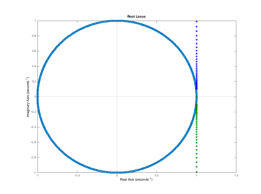
A complex plane (real along x-axis, imaginary along y-axis, showing the Unit Circle (blue) and the locations of the natural frequencies (green and purple) for increasing proportional gain for the LDE associated with Proportional Control of the Crane. Notice that the line of natural frequencies versus proportional gain. For K_p = 0, \lambda_1=\lambda_2 = 1, and as K_p increases, the natural frequencies lie on a line outside the unit circle. Therefore, the natural frequencies at EVERY gain have magnitude larger than one, so the proportional controller for this crane problem is NEVER stable.

The above result demonstrates the value of a the mathematical analysis, to show that using proportional feedback will never result in a stable system, regardless of the gain. But there is also a simple intuition. The problem with proportional controller is that it insures that the crane acceleration goes to zero when the crane is at the desired position, but does not insure that the crane's velocity is zero. So the crane has zero acceleration but NOT zero velocity when at the right spot, and will NOT STOP.

To stabilize the controller, we can try to more rapidly decelerate the crane as it approaches the desired position, to drive the velocity to zero and avoid overshooting. To accomplish this more rapid deceleration, consider adding another feedback term, proportional to the change in error,

where the position error, e[n] is defined as

The intuition for using the change in error from one sample to the next is most easily understood for the case of a constant desired position (d_{in}[n] = d_{in}[n-1]). In this case, the error difference is the approximately the negative of the crane velocity,

So, Delta feedback reduces the crane acceleration when the velocity is large! Exactly what we need, a controller term that also drives the velocity to zero while driving the position error to zero . The result, we hope, is that the crane gets to the right position and with zero velocity, and stops.

In order to determine if our intuition is correct, we will need to evaluate the natural frequencies of the crane with proportional plus this delta (PD) feedback. To do so, we substitute the PD controller for the acceleration in the equations for the crane,

Reorganizing, and assuming d_{in}[n] =0, because we only need the homogenous equation for natural frequencies,

Now we have a third-order difference equation, and must find the roots of a cubic equation to determine the natural frequencies. There is an analytic formula for roots of cubics, but it is complicated to apply, and we suggest using a numerical procedure (like the roots function in matlab or numpy). As an example, if Delta T = 0.01, K_p = 10 and K_d = 0.5, the natural frequencies are approximately 0.997 + 0.0316 j, 0.997 - 0.0316 j and 0.005, all less than one in magnitude, so the system is stable. And its step response (normalized) oscillates, but does stabilize.

A normalized step response for the pd controller applied to the crane system, for proportional gain = 10 and delta gain = 0.5.

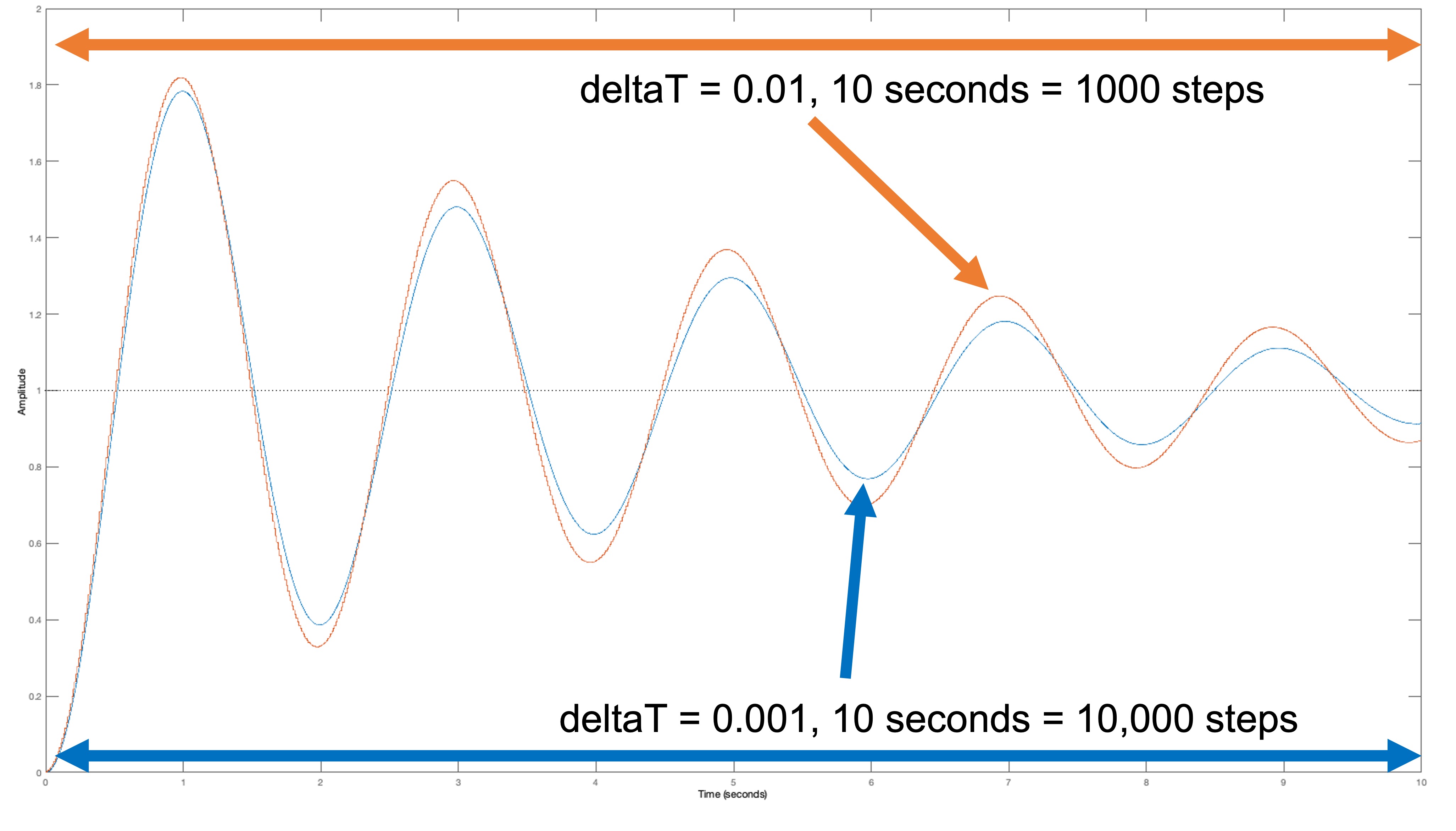
The above coefficients result in stable, but oscilitory behavior. Can we improve performance? For the first-order speed control problem, we could dramatically improve stability by increasing the sample rate (decreasing \Delta T). Does reducing \Delta T = 0.01 to \Delta T = 0.001 improve the controller behavior in this case?

Determine the natural frequencies of the crane control system for the \Delta = 0.001 case and enter them (in any order) in the boxes below. (NOTE: Use j=\sqrt {-1} and enter decimal representations in place of fractions wherever necessary. For example, the complex number \frac{7}{8}+\frac{1}{2}j is entered as 0.8750+0.5000j.) Note: you must enter the answer as a Python list for the autochecker to work, for example, '[0.9003+0.1021j,0.9003-0.1021j,0.5005]').

If you examine the natural frequencies for the \Delta T = 0.001 case, the situation APPEARS worse, because the largest magnitude \lambda's for the \Delta T = 0.001 case are slight larger than for the \Delta T = 0.01 case. However, if one plots step responses from both cases on the same time axis (as below), they appear to be nearly identical.

How well can you do with PD control? Since the crane system with PD feedback is identical, other than a scaling factor, to the system for controlling copter-levitated arm position, we will defer addition analysis to the Lab. And as we will see in lab, Root-Locus plots will help us optimize our designs.