Oscillating Second Order Systems

The questions below are due on Thursday February 29, 2024; 10:30:00 PM.

You are not logged in.
Please Log In for full access to the web site.
Note that this link will take you to an external site (https://shimmer.mit.edu) to authenticate, and then you will be redirected back to this page.

1) Sign-Flipped Fibonacci, big implications from a small change

Consider modifying the Fibonacci LDE by a single sign change, as in

y[n] = y[n-1] - y[n-2]

As we will see, things turn out quite a bit differently. Lets follow the procedure to find the natural frequencies of this LDE. First we will assume we have a solution of the form y[n] = c\lambda^n. Plug this in to the LDE to get

c\lambda^n = c\lambda^{n-1} - c\lambda^{n-2}.

Divide by c\lambda^{n-2} to find that,

\lambda^2 = \lambda - 1.

If we apply the quadratic formula to determine the natural frequencies we get:

\left(\lambda_1,\lambda_2\right) = \frac{1 \pm \sqrt{1-4}}{2} = \frac{1 \pm \sqrt{-3}}{2} = \frac{1}{2} \pm \frac{\sqrt{-3}}{2}

The natural frequencies in this case have terms where the negative sign is inside the square root, and this means the natural frequencies are complex numbers (see below). Regardless, we can blindly proceed, and produce a formula for the homogenous solution of this LDE

y[n] = c_1\cdot\left(\frac{1}{2} + \frac{\sqrt{-3}}{2}\right)^n + c_2\cdot\left(\frac{1}{2} - \frac{\sqrt{-3}}{2}\right)^n \\

Let's look at the result for a few times steps:

y[0] = c_1\cdot\left(\frac{1}{2} + \frac{\sqrt{-3}}{2}\right)^0 + c_2\cdot\left(\frac{1}{2} - \frac{\sqrt{-3}}{2}\right)^0 = \fbox{$c_1 + c_2$}

y[1] = c_1\cdot\left(\frac{1}{2} + \frac{\sqrt{-3}}{2}\right)^1 + c_2\cdot\left(\frac{1}{2} - \frac{\sqrt{-3}}{2}\right)^1 = \fbox{$\left(c_1+c_2\right)\cdot\frac{1}{2} + \left(c_1-c_2\right)\cdot\frac{\sqrt{-3}}{2}$}

y[2] = c_1\cdot\left(\frac{1}{2} + \frac{\sqrt{-3}}{2}\right)^2 + c_2\cdot\left(\frac{1}{2} - \frac{\sqrt{-3}}{2}\right)^2

= c_1\cdot\left(\frac{1}{4} + \frac{-3}{4} + \frac{\sqrt{-3}}{2}\right) + c_1\cdot\left(\frac{1}{4} + \frac{-3}{4} - \frac{\sqrt{-3}}{2}\right)

= \fbox{$(c_1+c_2)\cdot\frac{-1}{2} + (c_1-c_2)\cdot\frac{\sqrt{-3}}{2}$}

The natural frequencies have negative signs inside square roots and are therefore complex, and this might seem impossible. The difference equation has real coefficients and the initial condition is real, so the solution must also be real. How can a solution be the weighted combination of powers of complex natural frequencies, and still be real?

Carefully tracking the real and imaginary parts of c_1 and c_2 yields the answer. For example, if c_1 = c_2, then the coefficient in front of the problematic term (the one with the square root of a negative number) will be zero, and the solution will be real. There are other possibilities for c_1 and c_2, as we will see after a brief digression to review complex numbers. After that, things go surprisingly smoothly. Well, not really that smoothly, there are a lot of oscillations.

2) A Brief Reminder about Imaginary and Complex Numbers

We will use the symbol j rather than i to denote the square root of negative one. Mathematicians and physicists usually use i but engineers, particularly electrical engineers, use j because the variable i usually denotes electric current.

Note that if j \equiv \sqrt{-1}, then j^2 = \sqrt{-1}^2 = -1,

j^3 = \sqrt{-1}^3 = \sqrt{-1}^2\cdot\sqrt{-1} = -1\cdot\sqrt{-1} = -j,

and

j^4 = j^2\cdot j^2 = 1.

In general, an imaginary number is the product of a real scalar and j. For example \sqrt{-4} = 2\sqrt{-1} = 2j, or 0.7\cdot j = 0.7\sqrt{-1}. To add and subtract imaginary numbers, one just adds or subtracts the scalars, as in -7.3j+.7j = (-7.3+0.7)j = -6.7j. Gathering terms to simplfy expressions of imaginary numbers is similarly straight-forward.

2.1) Complex Numbers

Products of real numbers are purely real, the product of a real and an imaginary number is purely imaginary, and the product of two imaginary numbers is purely real. In general, the sum of, or difference between, a real and imaginary number is neither purely real nor purely imaginary, but is a complex of the two. For brievity, we refer to such real-imaginary complexes as complex numbers, and determining products and powers of such numbers can become tedious without a few tricks.

Consider the complex number z = 1+2j. Computing z+z is simple enough,

z+z = (1+2j)+(1+2j) = 1+1+2j+2j = 2+4j.

or given the generic a, b, c, and d form,

(a+bj)+(c+dj) = (a+c) + (b+d)j.

In general, when summing complex numbers, the real part is the sum of the sum of the real parts and the imaginary part is the sum of the sum of the imaginary parts.

There is no correspondingly simple formula for computing products of complex numbers, at least not for complex numbers represented in Cartisian ( a + bj) form. Even multiplying a pair of Cartisian-form complex numbers requires several steps,

(a+bj)\cdot(c+dj) = ac + ad\cdot j+bc\cdot j + bdj^2 = ac-bd+(ad+bc)j,

and raising them to high integer powers can be quite complicated. As we will see below, if we represent complex numbers in magnitude-angle form, products and powers are much easier to compute.

Answering Questions with Complex Numbers

Use this example to become familar with the format used to represent complex numbers when answering on-line questions.

If x = 7 and z = 3+4j, what is x+z? (NOTE: Use j=\sqrt {-1} and enter decimal representations in place of fractions wherever necessary. For example, the complex number \frac{7}{8}+\frac{1}{2}j is entered as 0.875+0.5j.)

If x = 7 and z = 3+4j, what is x\cdot z?

3) Return to Modified Fibonacci

Writing the natural frequencies of our modified Fibonacci LDE as complex numbers, we see that

\frac{1}{2} \pm \frac{\sqrt{3}j}{2},

are two complex conjugate natural frequencies. That is, when the real part of two complex numbers are equal, and their imaginary parts are equal in magnitude but opposite in sign, the two numbers are called complex conjugates. The sum of complex conjugates is purely real, the difference, purely imaginary.

We can look back at the general solution we had before and the solutions at specific time steps

y[0] = c_1 + c_2

y[1] = \left(c_1+c_2\right)\cdot\frac{1}{2} + \left(c_1-c_2\right)\cdot\frac{\sqrt{3}j}{2}

y[2] = (c_1+c_2)\cdot-\frac{1}{2} + (c_1-c_2)\cdot\frac{\sqrt{3}j}{2}

Before we said that if c_1 = c_2, y[n] would always be real. Now we know a little more and ought to revise that statement. So long as the real part of c_1 - c_2 is zero, then y[n] will always be real. An imaginary component of that difference will multiply by the imaginary component of the natural frequencies. However if we allow c_1 \text{ and } c_2to be complex, then c_1 + c_2 might have a complex component. To have a purely real y[n] we therefore need to constrain the imaginary components of c_1 and c_2 such that their sum is equal to zero. If we let c_1 = a+bj then c_2 = a-bj.

This is of course not a rigorous proof. We have only looked at the zeroth first and second time steps. However, this property (complex conjugate coefficients for complex conjugate natural frequencies producing real valued sequences) holds true for all n.

An example constraint

As an example of this not being an issue, suppose our initial conditions are still y[0]= 0 and y[1]= 1 as before. A quick check will assure you that y[0] = 0 results in the constraint that c_1 = - c_2. And satisfying the y[1] = 1 constraint leads to

y[1] = c_1 \left(\frac{1 + \sqrt {3}j}{2}\right)^1 + c_2 \left(\frac{1 - \sqrt {3}j}{2}\right)^1=1

c_1=\frac{-j}{\sqrt {3}}

The values of the sequence are then given by

y[n] = \frac{-j}{\sqrt {3}} \left(\frac{1 + \sqrt {3}j}{2}\right)^ n + \frac{j}{\sqrt {3}} \left(\frac{1 - \sqrt {3}j}{2}\right)^ n

which you can verify is always real valued. (Of course, if you compute this numerically, you might end up with vanishingly small imaginary parts.)

Why are the sequences always real, even when the natural frequencies are complex? Part of the reason is that a_1 and a_2 are real, so \lambda _1 and \lambda _2 are roots of a quadratic with real coefficients, and therefore must both be real, or must form a complex conjugate pair (a+bj and a-bj). And if the roots, or natural frequencies, form a complex conjugate pair, then constraining c_1 and c_2 to be a complex conjugate pair guarantees that the resulting sequence will be real. But even with the complex conjugate constraint on c_1 and c_2, there will still be two degrees of freedom (one real part and one imaginary part for the complex conjugate pair), just enough to match any two real values for y[0] and y[1].

Consider the following difference equation in standard form,

y[n] = -\frac{3}{2}y[n-1]-\frac{5}{8}y[n-2]

Determine the natural frequencies of the system and enter them (in any order) in the boxes below. (NOTE: Use j=\sqrt {-1} and enter decimal representations in place of fractions wherever necessary. For example, the complex number \frac{7}{8}+\frac{1}{2}j is entered as 0.875+0.5j.) Note: you must enter the answer as a Python list for grading to work)

Let the solution to the difference equation

y[n] = a_1 y[n-1] + a_2 y[n-2],

y[n] = c_1(1-j)^ n + (5+j)(1+j)^ n

where j=\sqrt {-1}.

Assuming y[n] is real for all n, determine a_1, a_2, and c_1. TAKE NOTE: Use j=\sqrt {-1} and enter decimal representations in place of fractions wherever necessary. For example, the complex number \frac{7}{8}+\frac{1}{2}j is entered as 0.875+0.5j.

a_1=

a_2=

Answers are analyzed as Python3 values. In Python you need to make sure to always specify a number with your complex term. So if you want to enter 14+j, you need to enter: 14+1j

c_1=

4) Polar Form

So far we have learned that systems can have complex natural frequencies, but what are their implications? Hopefully this section will bring this to light. Suppose a pair of natural frequencies for a difference equation are complex. Since the difference equations we will consider have real coefficients, for us, complex natural frequencies will always appear in complex-conjugate pairs, a point we will return to later. At the moment, we will be concerned with computing the powers of a complex natural frequency, needed when evaluting the difference equation solution.

Suppose one of natural frequencies is complex, \lambda = a+bj , where j = \sqrt{-1}. Then what is \lambda^n in terms of a and b? For example, suppose n = 4, then

\lambda^4 = (a+bj)^4 = (a+bj)(a+bj)(a+bj)(a+bj) = (a^2 - b^2 + 2abj)(a^2 - b^2 + 2abj) = ....,

well, a very complicated expression. And one that does not lend much insight about the properties of the difference equation solution, such as the solution decaying, or growing, or oscillating.

Representing complex natural frequencies as a + bj is not the most convenient form to represent a complex number when computing powers. As an alternative, think of the pair (a, b) as specifying a point in the two-dimensional plane. That is, the coefficient of the real part of the number, a , specifies a point on the x-axis, and the coefficient of the imaginary part of the number, b, specifices a point on the y-axis. Now imagine drawing a line from the origin of the coordinate system to our (a,b) point. As an example, consider the complex number a+bj \approx 2+j, shown in the complex plane Figure 1 below.

Complex c_1 \approx 2+j with magnitude \sqrt{5} and angle \approx \frac{\pi}{6.77} .

As can be seen from the Figure, a complex number a + bj can be represented by a magnitude and an angle, M, \Theta , where the magnitude is given by

M = \sqrt{a^2 + b^2},

the real part is given by

a = M \cos{\Theta},

the imaginary part is given by

b = M \sin{\Theta},

and the angle is given by

\Theta = \arctan{\frac{b}{a}}.

Note that

\frac{b}{a} = \frac{\sin{\Theta}}{\cos{\Theta}} = \tan{\Theta},

leading to the arctangent (or inverse tangent) formula above.

4.1) Evaluating Powers of Complex Natural Frequencies

The main advantage of the magnitude/angle form is the simpler formula for computing powers of a complex number, needed to compute difference equation solutions given complex natural frequencies. That is,

\lambda^n = (a+bj)^n = \left(M \; (\cos{\Theta} + j\sin{\Theta}) \right)^n = M^n \cdot (\cos{\Theta} + j\sin{\Theta})^n.

Is that really much simpler?

We need one more extraordinary fact, Euler's relation, which states

e^{j\Theta} = \cos{\Theta} + j\sin{\Theta},

and therefore

a+bj = Me^{j\Theta}

which we refer to as the polar form, or magnitude-angle form, of a complex number.

There are many ways proving Euler's relation, of which we offer none. Type it into your favorite search engine and you will find many proofs to choose from. What concerns us is the fact that \left( e^{c} \right)^n = e^{c \cdot n } for any c , even if it is complex. That means,

\left(e^{j\Theta} \right)^n = e^{j\Theta \;n} = \cos{\Theta \; n} + j\sin{\Theta \; n},

a relation that might make you question why you had to learn all those half and double angle formulas in trigonometry. You are welcome to forget them now.

Now consider squaring a complex number in the magnitude/angle representation,

\left(M e^{j \Theta }\right)^2= M e^{j \Theta } M e^{j \Theta }

=M^2 e^{j 2 \Theta }

And for arbitrary n, we have that

\left(M e^{j\Theta }\right)^ n = M^ n e^{j n \Theta }

which is not only easy to compute, but easy to reason about for large n.

For example, what happens to the n^{th} power of the magnitude/angle representation as n approaches \infty? The magnitude, M^ n, will grow or shrink depending on whether M is larger or smaller than one. And e^{j n \Theta } always has magnitude one, and only changes the relative contribution and signs of the real and imaginary parts. So when we represent a natural frequency as M e^{j \Theta }, we can easily answer questions about high powers of the natural frequency. If we are concerned with what a natural frequency tells us about the stability of the associated homogenous LDE, or want to know whether the associated sequence grows exponentially or decays to zero, then we need only compare the natural frequency's magnitude to one.

Regardless of whether natural frequencies are real or complex or positive or negative, if the magnitudes of both natural frequencies are greater than one, then any associated sequence will grow exponentially and the associated LDE is unstable. If both magnitudes are less than one, then any associated sequence will decay to zero, and the associated LDE is stable. And if the magnitude of one natural frequency is greater than one, and the other less than one, then the behavior of an associated sequence will depend on initial conditions, but the associated LDE is unstable. Consider a system modeled by the difference equation

y[n]= -2y[n-1]-y[n-2]

with initial conditions y[0]=1 and y[1]=-1.

Which of the following most accurately characterizes the long-time behavior of the system?

5) Computing Oscillation Period

Complex-conjugates c_1 \approx 2+j and c_2 \approx 2-j, each with magnitude \sqrt{5} , and angles \approx 0.46 and \approx -0.46 respectively.

In second-order homogenous LDEs, we only have two natural frequencies, \lambda _1 and \lambda _2. And since the LDE coefficents are real, if \lambda_1 is complex, then \lambda_2 is its complex conjugate, meaning both have equal magnitude but opposite sign imaginary parts (see Figure 2 above). More specifically,

\lambda_1 = Me^{j\Theta} \;\;\; \lambda_2 = Me^{-j\Theta}.

When it comes to computing the solution to a difference equation with real coefficients and real initial conditions, we can say even more. That is, y[n] in

y[n] = c_1 \lambda_1^n + c_2 \lambda_2^n

must be real, so if the natural frequencies are a complex conjugate pair, then c_1 and c_2 must be a complex conjugate pair also. Using polar form for the \lambda's and the c's (e.g. \lambda_1 = Me^{j\Theta} and c_1 = M_ce^{j\Theta_c}),

y[n] = M_ce^{j\Theta_c}M^ne^{j\Theta \;n} + M_ce^{-j\Theta_c}M^ne^{-j\Theta \; n}

where \lambda_2 = Me^{j\Theta} , the complex conjugate of \lambda_1,and c_2 = M_ce^{-j\Theta_c} , the complex conjugate of c_1.

Simplifying,

y[n] = M_c\cdot M^n \left(e^{j\Theta_c + \Theta \;n} + e^{-j(\Theta_c + \Theta \;n)} \right).

Euler's relation can be used to show e^{j\Theta} + e^{-j\Theta} = 2\cos{\Theta} , and therefore

y[n] = 2 M_c\cdot M^n \cos{(\Theta \;n + \Theta_c)}.

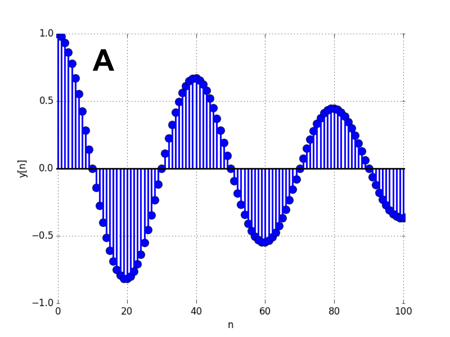
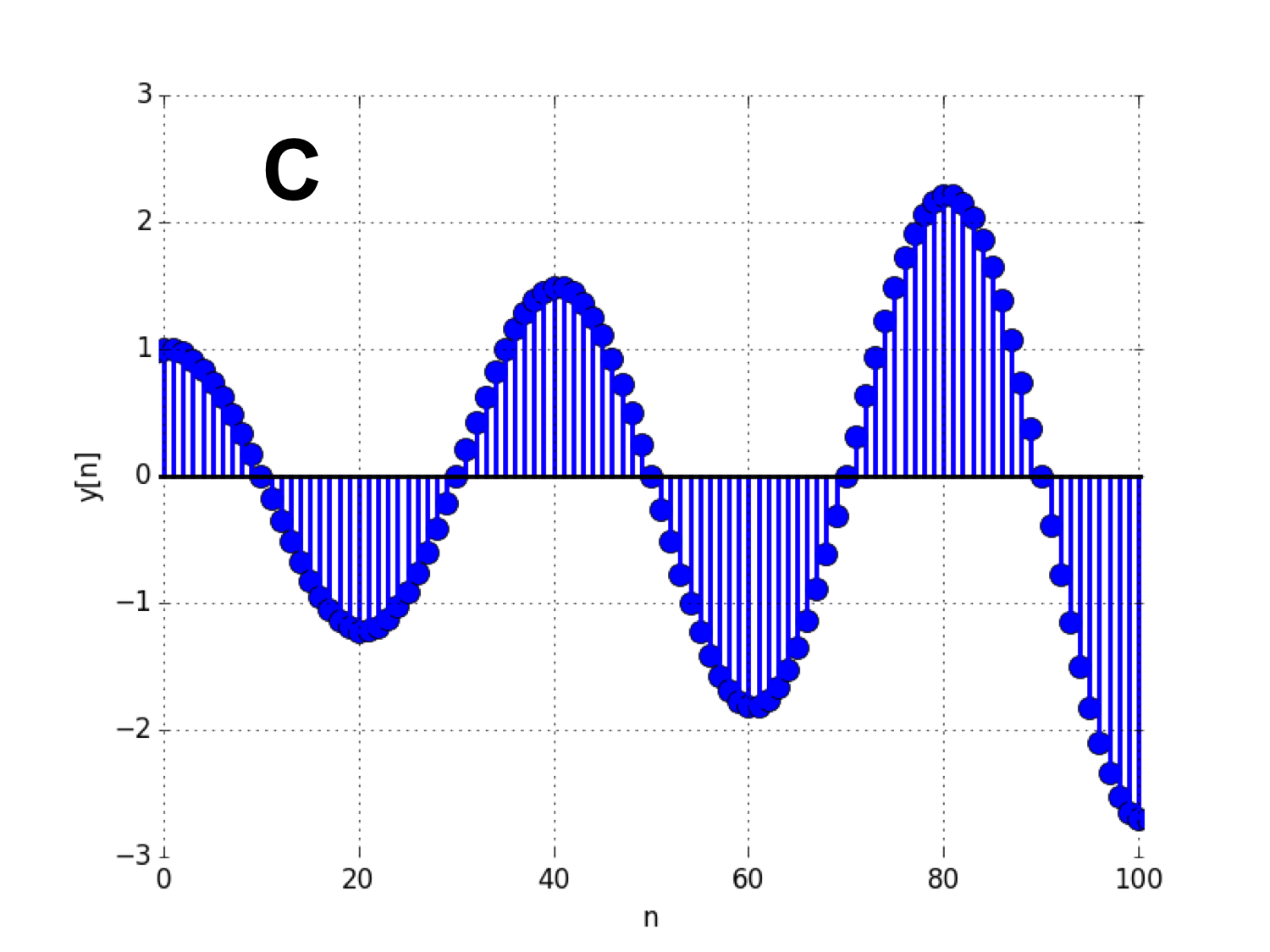
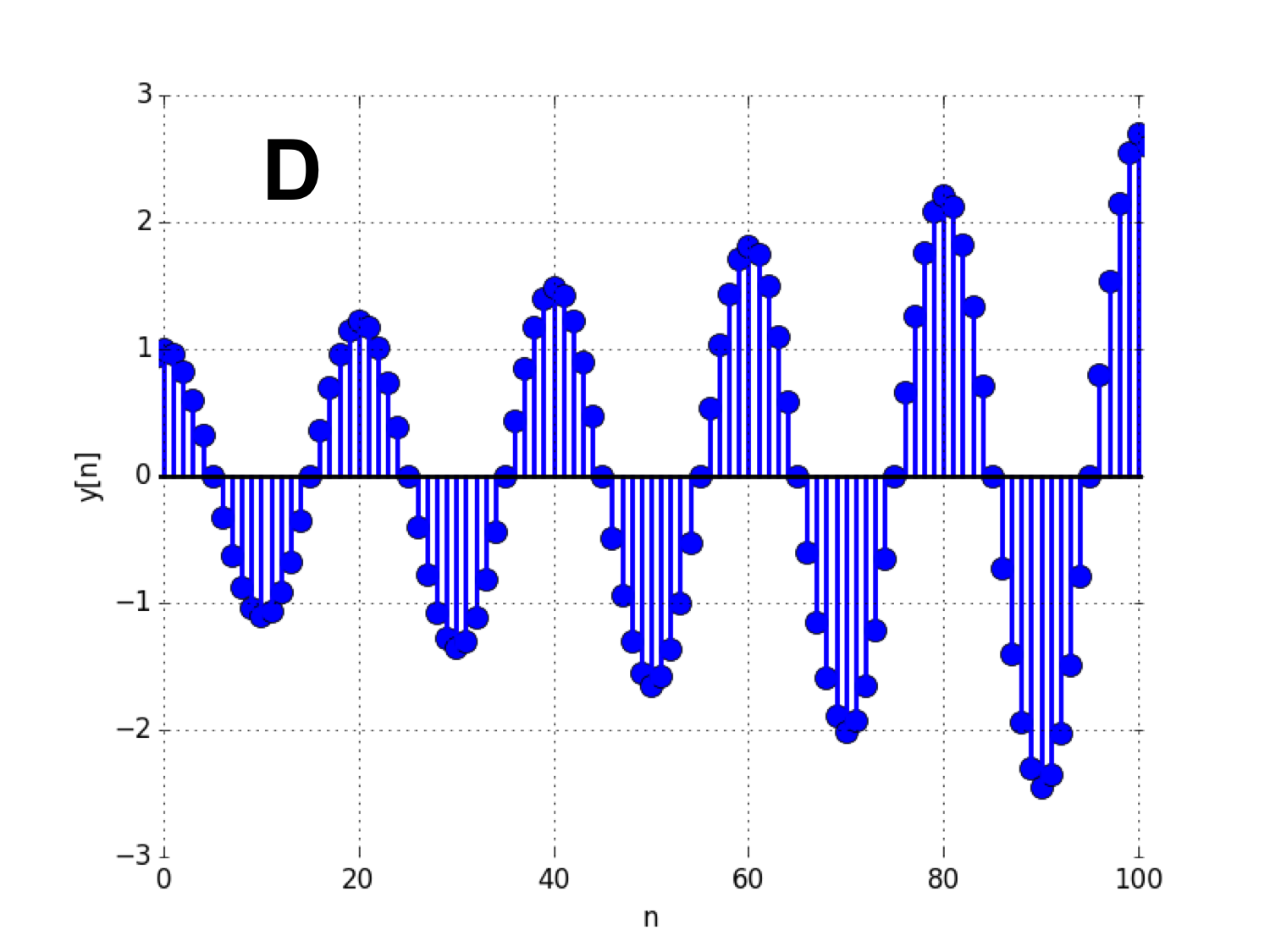
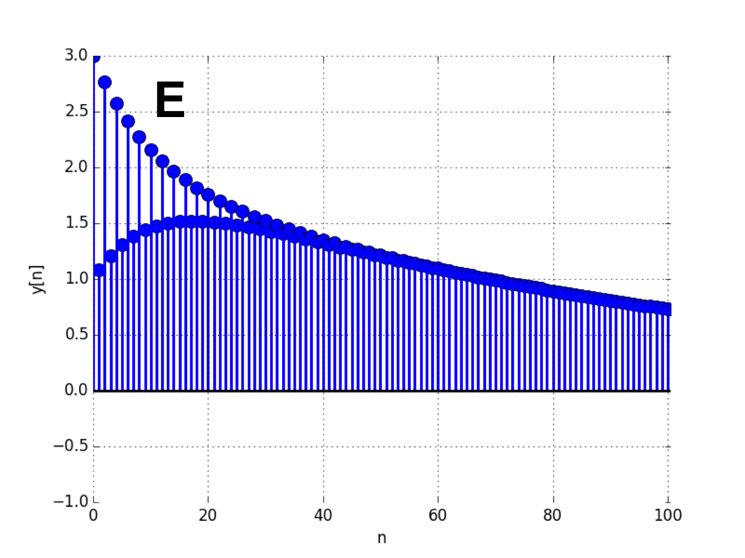
Summarizing, when a difference equation has a complex-conjugate pair of natural frequencies, then the solution to the difference equation will oscillate with a period of \frac{2 \pi}{\Theta} samples. We will examine such solutions in the following problem and in lab.

For the following problems, consider the sequences y[n] shown in the plots below. Each sequence is a solution to a second-order LDE.

Which of the plots above correspond to non-real frequencies? (Select all that apply.)

Which of the plots correspond to stable difference equations? (Select all that apply.)

Which of the plots correspond to natural frequencies with angle \pi /10? (Select all that apply.)

Which of the plots have at least one negative real natural frequency? (Select all that apply.)

At least one of the plots corresponds to natural frequencies of 0.99 and 0.9? Which ones?