Second Order Homogenous Linear Difference Equations

The questions below are due on Thursday February 29, 2024; 10:30:00 PM.

You are not logged in.
Please Log In for full access to the web site.
Note that this link will take you to an external site (https://shimmer.mit.edu) to authenticate, and then you will be redirected back to this page.

1) Crane Mutiny Example

Crane Seeking a Beacon

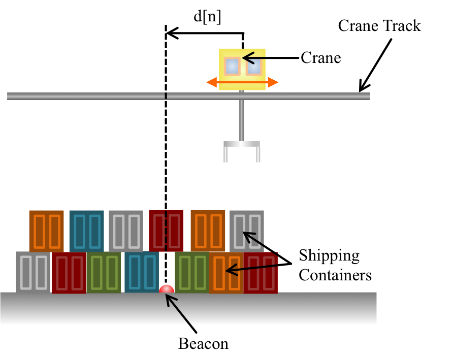
A heavy cargo crane travels on track above a buried beacon, and measures its signed distance to the beacon 100 times a second (by signed distance, we mean that the distance is positive if the crane has not yet reached the beacon and negative if the crane has traveled past it). A human operator usually drives the crane and parks it just above the beacon. The crane then keeps itself in place automatically by always accelerating towards the beacon at a rate proportional to its distance from the beacon. On one unfortunate day, the operator noticed that the crane seemed to be "rocking" back and forth over the beacon, and tried to fix the problem by flipping the sign of the distance sensor. The crane almost immediately sped off down the track, halted only by the quick-thinking operator, who shut down the crane. Why did this happen?

In the previous prelab, we assumed that we could control the crane by sending it velocity commands, which led to a first-order difference equation model. A more realistic model would be to assume that we can send the Crane acceleration commands, and that will lead to a more complicated higher-order difference equation model. We will start in the same way, and will represent the crane's measured distance to the beacon as a sequence, d, where d[n] is the n^{th} measured distance. Then d[n] can be related to d[n-1] by

d[n] - d[n-1] \approx 0.01 v[n-1]

where 0.01 is the number of seconds between distance measurements, v[n-1] is the crane velocity at the time of the (n-1)^{th} distance measurement, and we note that the relationship is approximate because the velocity of an accelerating crane varies continuously. Since crane acceleration is proportional to measured distance, it does not vary between samples, so we have an exact relation between velocity and acceleration. That is,

v[n] - v[n-1] = 0.01 a[n-1] = -0.01 \gamma d[n-1]

where a[n-1] is the crane acceleration at the time of the (n-1)^{th} distance measurement, and \gamma is the proportionality factor relating acceleration to measured distance. There are now two sequences, v and d, and two first-order LDEs. We would like to determine natural frequencies, but of what? If you continue to study control theory, you will learn that transform techniques considerably simplify solving this problem. But for now, we will lean on some of the LDE properties we have learned.

1.1) Constructing the model

To begin, consider that an LDE holds for all n, so we can shift the index by one and write equivalent LDEs for d and v,

d[n-1] - d[n-2] \approx 0.01 v[n-2]

and

v[n-1] - v[n-2] = -0.01 \gamma d[n-2]

Subtracting the shifted from the unshifted LDE for d yields a second-order LDE for d and v,

\left(d[n] - d[n-1]\right) - \left(d[n-1] - d[n-2] \right) \approx 0.01 \left(v[n-1] - v[n-2]\right)

The shifted LDE for v can be used to eliminate velocity, and after that elimination,

\left(d[n] - d[n-1]\right) - \left(d[n-1] - d[n-2] \right) \approx - (0.01)^2 \gamma d[n-2]

Gathering terms considerably simplifies the equation, and the result is a second-order homogenous LDE for d[n] alone,

d[n] - 2d[n-1] + \left(1+(0.0001 \gamma )\right) d[n-2] \approx 0.

So now we need to learn about solving higher order difference equations, and we will start with a classic example, the Fibonacci series.

2) Fibonacci as LDE

Consider the Fibonacci sequence, in which the next element in the sequence is the sum of the previous two. The sequence has a second-order LDE description,

y[n] = y[n-1] + y[n-2].

Since the LDE for the Fibonacci sequence uses the previous two values, we refer to its associated LDE as second-order. If we specify y[0] and y[1], which we often refer to as initial conditions, then we can use the above difference equation to iteratively compute y[n] for all n \ge 2.

For example, to generate the classic Fibonacci numbers, set y[0] = 0 and y[1] = 1, and repeatedly apply the above formula with n =2 , then n=3, n=4, and so on, to determine y[2]=1, y[3]=2, y[4]=3, y[5]=5, ... etc. In general, given an LDE and enough initial conditions, it is easy to explicitly enumerate the rest of the sequence values.

These questions refer to the Fibonacci difference equation

y[n] = y[n-1] + y[n-2].

If you pick initial conditions y[0] = 8 and y[1] = 13 for the above difference equation, what will be true about the generated sequence y[2], y[3], y[4], y[5], ... ? Please list all that apply below (separated by commas).
- A: The sequence entries will grow without bound.
- B: The sequence entries match the values of a shifted Fibonacci sequence.
- C: \lim_{n \rightarrow \infty} \frac{y[n]}{y[n-1]} > 2.

Suppose the initial conditions for the difference equation are given by two constants, A and B , where y[0] = A and y[1] = B . What will be true about the generated sequence y[2], y[3], y[4], y[5], ... ? Please check all that apply.

A: If A is negative and B is positive, and |A| \gt B , then it is guaranteed that y[n] \lt 0 for all n \gt 2 .
B: If A is negative and B is positive, and |A| \gt 2\cdot B , then it is guaranteed that y[n] \lt 0 for all n \gt 2 .
C: If A is positive and B is negative, and A \lt |B| , then it is guaranteed that y[n] \lt 0 for all n \gt 2 .
D: If A is positive and B is negative, and |A| \gt |2\cdot B |, then it is guaranteed that y[n] \lt 0 for all n \gt 2 .

3) Quadratic Equation for Natural Frequencies

Sequences described by second-order homogenous LDEs, like the Fibonacci sequence, have the property that y[n] is given by a weighted combination of y[n-1] and y[n-2]. Their general form is

y[n] = a_1 y[n-1] + a_2 y[n-2].

To uniquely specify the sequence associated with the second-order difference equation, it is necessary to specify two initial conditions, y[0] and y[1]. First-order difference equations only require one initial condition, but a more problematic difference is that an explicit solution is not as readily apparent for the second-order homogenous LDE as it was in the first-order case. We will need a strategy for finding it.

To begin, we know that the general solution to the first-order homogenous LDE,

y[n] = \lambda y[n-1]

y[n] = {\lambda}^n y[0]

and even though \lambda^n is not the solution to the second-order LDE unless a_2 = 0 (in which case \lambda = a_1), it does suggest a way to guess at the solution.

Suppose we assume that a second-order homogenous LDE has a solution of the form

y[n] = c \cdot \lambda^n,

and we then plug this assumed form back into the homogenous LDE to determine values for \lambda and c. Substituting y[n] = c \lambda ^ n into the general form for a second-order homogenous LDE yields

c \lambda ^ n = a_1 \cdot c \cdot \lambda ^{n-1} + a_2 \cdot c \cdot \lambda ^{n-2}.

Simplifying by dividing through by c \cdot \lambda ^{n-2} results in a quadratic equation for \lambda,

\lambda^2 = a_1 \lambda + a_2 \;\;\;\;\text{ or } \;\;\;\;\lambda ^2 - a_1 \lambda - a_2 = 0,

which nearly always has two distinct solutions, the roots of the quadratic equation on the right side of the above. And the roots of the quadratic equation are explicit functions of a_1 and a_2 , given by the well-known quadratic formula:

(\lambda _1, \lambda _2) = \frac{a_1 \pm \sqrt {a_1^2 + 4 a_2}}{2}.

Assumption: In the following approach for solving second-order homogenous LDEs, we implicitly assume that the quadratic equation for \lambda has two distinct roots, which we will later refer to as two distinct natural frequencies. It can happen that \lambda _1 = \lambda _2, and in this generally-rare repeated-root case, the approach below must be replaced with a distractingly complicated alternative. In our case, we are the ones creating the models and designing the controllers, so it is particularly easy for us to avoid the rare repeated-root case.

By solving the quadratic equation, we found a pair \lambda_1 and \lambda_2 such that \lambda_i^2 = a_1 \lambda_i + a_2, for i = {1,2} . As a result, we know that the second-order homogenous LDE will be satisfied by y[n] = c_1 \lambda_1^n or by y[n] = c_2 \lambda _2^n, and for any values of c_1 and c_2 we care to choose. For this reason, we refer to \lambda _1 and \lambda _2 as the two natural frequencies for the second-order homogenous LDE, they characterize how the difference equation behaves when there is no external input.

Like the first-order case, natural frequencies give us whole families of sequences that satisfy the homogenous LDE. But unlike the first-order case, we have two families that can be used in any combination. That is, y[n] = c_1 \lambda _1^ n + c_2 \lambda _2^ n satisfies the second-order homogenous LDE, for any c_1 and c_2. That there is such a rich collection of solutions to the LDE is easily shown by plugging in and verifying. That is, we need to verify that

y[n] = c_1 \lambda _1^n + c_2 \lambda_2^n

implies that

y[n] - \left( a_1 y[n-1] + a_2 y[n-2] \right) = 0.

Using the assumed form for y[n],

y[n-1] = c_1 \lambda _1^{n-1} + c_2 \lambda_2^{n-1}

and

y[n-2] = c_1 \lambda _1^{n-2} + c_2 \lambda_2^{n-2},

which implies

y[n] - \left( a_1 y[n-1] + a_2 y[n-2] \right) = c_1 \lambda _1^n + c_2 \lambda_2^n - \left( a_1 \left( c_1 \lambda_1^{n-1} + c_2 \lambda_2^{n-1} \right) + a_2 \left( c_1 \lambda_1^{n-2} + c_2 \lambda_2^{n-2} \right) \right).

By combining terms with a common \lambda_i, we can determine an equivalent verification. That is, we need only verify that

\left( c_1 \lambda_1^n - a_1 c_1 \lambda_1^{n-1} - a_2 c_1 \lambda_1^{n-2} \right) + \left( c_2 \lambda_2^n -a_1 c_2 \lambda_2^{n-1} - a_2 c_2 \lambda_2^{n-2} \right)

= c_1 \lambda_1^{n-2} \left( \lambda_1^2 - a_1 \lambda_1 - a_2 \right) + c_2 \lambda_2^{n-2} \left(\lambda_2^2 - a_1 \lambda_2 - a_2 \right)

is equal to zero for any c_1 and c_2. But we know that each of the above parenthesized terms is zero, and therefore their weighted sum is zero, because setting those parenthesized terms to zero is how we determined \lambda_1 and \lambda_2 in the first place.

Suppose the solution to a second order difference equation is

y[n] = c_1 \cdot 3^n + c_2 \left(\frac{-1}{2}\right)^n.

If y[n] goes to zero as n \rightarrow \infty , what is c_1 ?

If y[n] \ge 0 for all n \ge 0 and c_2 = 3 , then what is the smallest possible value for c_1 (give answer as a decimal number)?

For what values of a_1 and a_2 will y[n] = a_1 y[n-1] + a_2 y[n-2]?

What is the value of a_1:

...and a_2:?

For the following problems, consider the second-order linear difference equation

y[n] = a_1 y[n-1] + a_2 y[n-2],

with the solution

y[n] = 10(-2)^ n + 5(-1)^n.

Determine a_1, a_2, y[0], and y[1].

a_1=

a_2=

y[0]=

y[1]=

4) Matching Initial Conditions

Now that we have the two natural frequencies, there is the matter of initial conditions. How to incorporate the initial conditions is best seen by example, so we will examine solving the second-order homogenous LDE for the Fibonacci sequence. Since the next value in the Fibonacci sequence is the sum of the previous two,

y[n] = y[n-1] + y[n-2],

or a_1 = a_2 = 1 in our general second-order homogenous LDE.

Using the quadratic formula above, we find that the Fibonacci LDE has two distinct natural frequencies,

(\lambda _1, \lambda _2) = \frac{1 \pm \sqrt {5}}{2},

therefore any sequence of the form

y[n] = c_1 \left(\frac{1 + \sqrt {5}}{2}\right)^ n + c_2 \left(\frac{1 - \sqrt {5}}{2}\right)^ n,

will satisfy the Fibonacci LDE.

In order to produce the classical Fibonacci sequence, we need to find values for c_1 and c_2 so that y[0] = 0 and y[1]= 1. To start, consider how y[0] = 0 constrains c_1 and c_2,

y[0] = c_1 \left(\frac{1 + \sqrt {5}}{2}\right)^0 + c_2 \left(\frac{1 - \sqrt {5}}{2}\right)^0=0

c_1 + c_2=0

c_1=-c_2

Including the constraint from y[1] = 1,

y[1] = c_1 \left(\frac{1 + \sqrt {5}}{2}\right)^1 + c_2 \left(\frac{1 - \sqrt {5}}{2}\right)^1=1

c_1 \frac{1 + \sqrt {5}}{2} - c_1 \frac{1 - \sqrt {5}}{2}=1

c_1 ((1 + \sqrt {5}) - (1 - \sqrt {5}))=2

c_1 2 \sqrt {5}=2

c_1 = \frac{1}{\sqrt {5}}

So, the final equation for the Fibonacci sequence is

y[n] = \frac{1}{\sqrt {5}} \left(\frac{1 + \sqrt {5}}{2}\right)^ n - \frac{1}{\sqrt {5}} \left(\frac{1 - \sqrt {5}}{2}\right)^ n\; \; .

Evaluating the numeric constants (approximately)

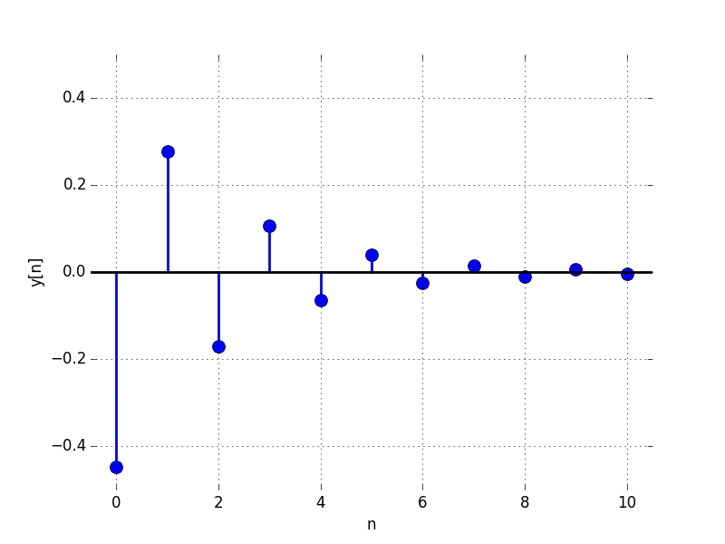
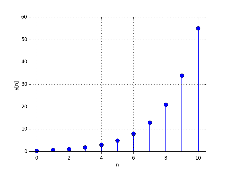
y[n] = 0.44721 \cdot 1.618^ n - 0.44721 \cdot (-0.618)^ n

Plots of the two components of the Fibonacci sequence, and their sum. The component in the leftmost graph is due to the negative natural frequency, and we can clearly see its oscillation, but note that its magnitude is very small. The lower sequence is the sum of the first two, and we can clearly see that the exponential growth associated with the large positive natural frequency dominates, and reveals the familiar large n approximation for the Fibonacci sequence.

Are there values of y[0] and y[1] for which the sequence given by

y[n] = c_1 \left(\frac{1 + \sqrt {5}}{2}\right)^ n + c_2 \left(\frac{1 - \sqrt {5}}{2}\right)^ n

decays to 0 as n approaches \infty?

Select the most accurate response below:

	No. The first term has a natural frequency with magnitude greater than one.
	Yes. Any choices of y[0] and y[1] will cause the sequence to decay to zero.
	Yes. Any choice of y[0] and y[1] that force c_1=0 will result in the sequence decaying to zero.
	Yes. Any choice of y[0] and y[1] that force c_2=0 will result in the sequence decaying to zero.

Consider a system modeled by the difference equation

y[n]= -2y[n-1]-y[n-2]

with initial conditions y[0]=1 and y[1]=-1.

Which of the following most accurately characterizes the eventually (large n) behavior of the sequence y?

	y decays to zero
	y grows unbounded
	y oscillates between two values
	None of the above

5) Higher Order Homogenous Difference Equations

The approach for solving second-order homogenous LDEs can be easily generalized to arbitrary order. The general form for a homogenous LDEs of order k is

y[n] = a_1 y[n-1] + \ldots + a_k y(n-k).

To find solutions to the k^{th}-order homogenous LDE, one again assumes solutions of the form y[n] = c \lambda ^ n, and substitutes that form into the LDE to generate its characteristic equation,

\lambda ^ n - a_1 \lambda ^{n-1} - \ldots - a_k \lambda ^{n-k} = 0.

The roots of the characteristic equation, \lambda _1, \ldots , \lambda _ k, are the k natural frequencies of the LDE.

Given k initial conditions, and assuming k distinct natural frequencies, one can solve k linear equations in k unknowns,

y[0]=c_1 + \ldots + c_ k

y[1] = c_1\lambda_1 + \ldots + c_k \lambda _ k

\cdots

y[k-1] = c_1\lambda_1^{k-1} + \ldots + c_k \lambda _ k^{k-1}

to determine values for c_1, \ldots , c_k. Then the closed form representation for the values of the associated sequence is given by

y[n] = c_1\lambda_1^ n + \ldots + c_k \lambda _ k^ n

There are some complications in the higher-order case. The roots of higher-order polynomials are almost always computed numerically. And with more natural frequencies, there are more ways for repeated natural frequencies to make life complicated. For the case of control system design, difference equations of order higher than three are rarely used. Instead, one switches to state-space methods, a topic you will certainly learn if you continue studying control theory.