The Propeller Arm

The questions below are due on Thursday February 29, 2024; 10:30:00 PM.
 

1) The Propeller Arm

In the up-coming lab, we will start levitating the propeller(aka copter) arm and controlling its angular position. To design the controller, we will first model the arm using difference equations, and wrestling with this prelab problem is intended to build up your arm modeling muscle.

In the video below, we demonstrate (using an earlier version of the copter-levitated arm) trying to position the arm by changing the propeller speed. More specifically, the actor in the video first adjusts the direct motor command (which is changing the current in to the propeller motor) so that the arm hovers about 45^{\circ } below horizontal. Note that even after pushing the arm a small distance with a cardboard tube, the arm returns to its 45^{\circ } below horizontal position. When the actor tries to adjust the direct command to position the arm 45^{\circ } above horizontal, the arm's behavoir is, well mustn't spoil the suspense. Our goal will be to understand the arm's behavior using a second-order homogenous LDEs.

1.1) Balancing the arm

The video actor is using our browser-based GUI for the arm to increase or decrease the direct command, which increases or decreases the propeller motor current, and accelerates or decelerates the propeller rotation speed. If the propeller spins fast enough, the arm lifts, and the actor succeeds in positioning the arm about 45^{\circ } below horizontal, as in the picture below.

The actor then tries to position the arm about 45^{\circ } above horizontal, but fails.

1.1.1) What Happened?

It is not possible to find a value for the direct command that keeps the arm at 45^{\circ } above horizontal. Even if you force the arm to the right position, once you let go, the arm will fly away. In order to understand the why the behaviors of the down-pointed and up-pointed cases are so different, we will develop an LDE model for each case and examine the associated natural frequencies.

1.2) Balancing Forces

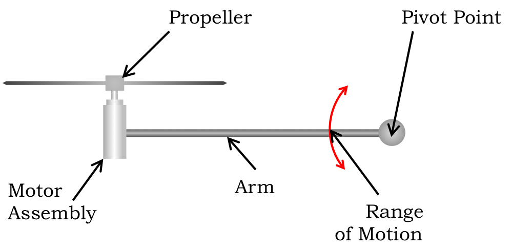
The copter-levitated arm is attached to a pivot (the shaft of the angle sensor) and is rotated by the gravity and copter forces at opposite end of the arm. The propeller force is generated by spinning a plastic propeller with a geared motor. Increasing the current to the motor causes the propeller to spin faster, thereby increasing its contribution to the rotation force.

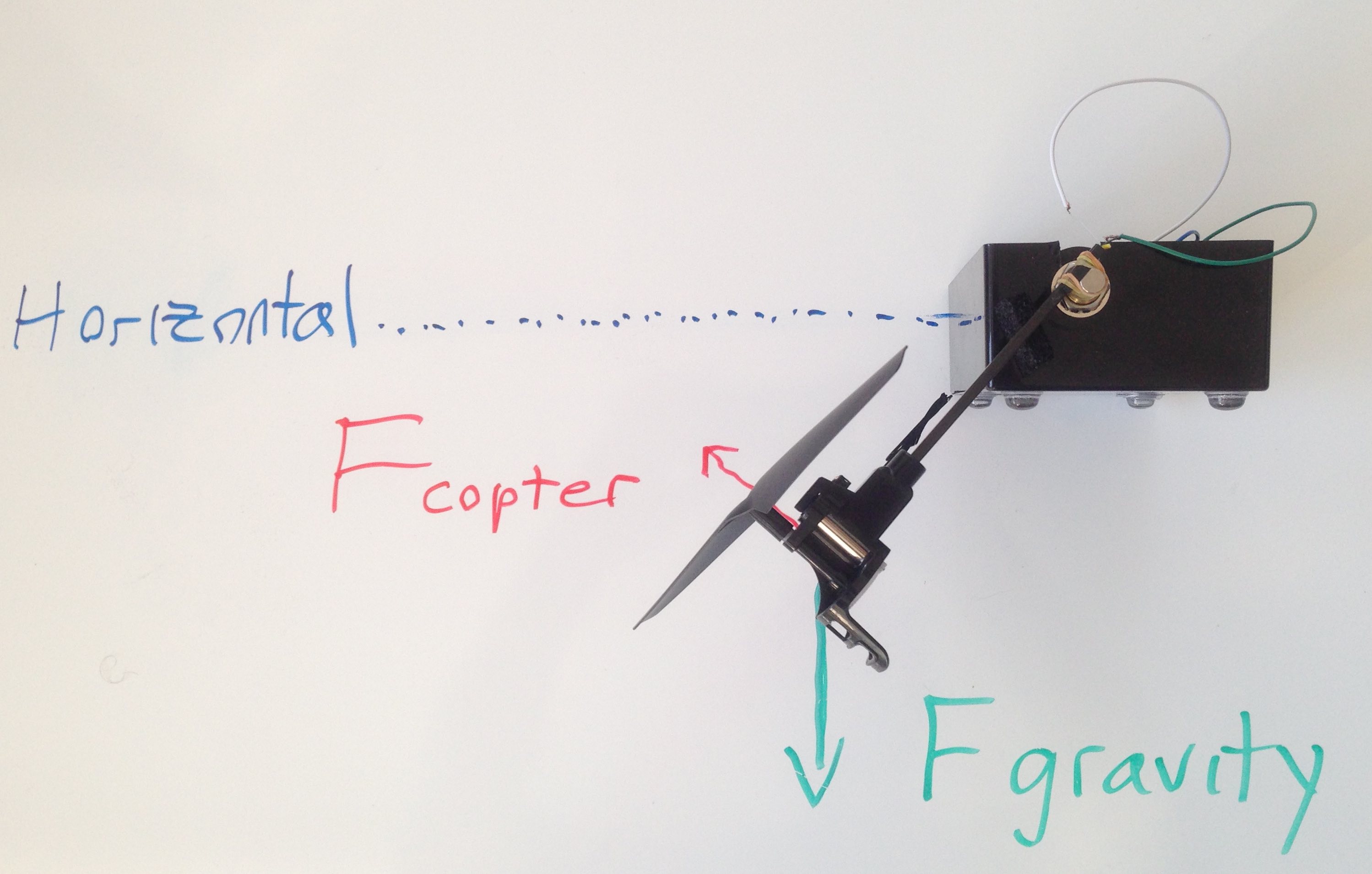
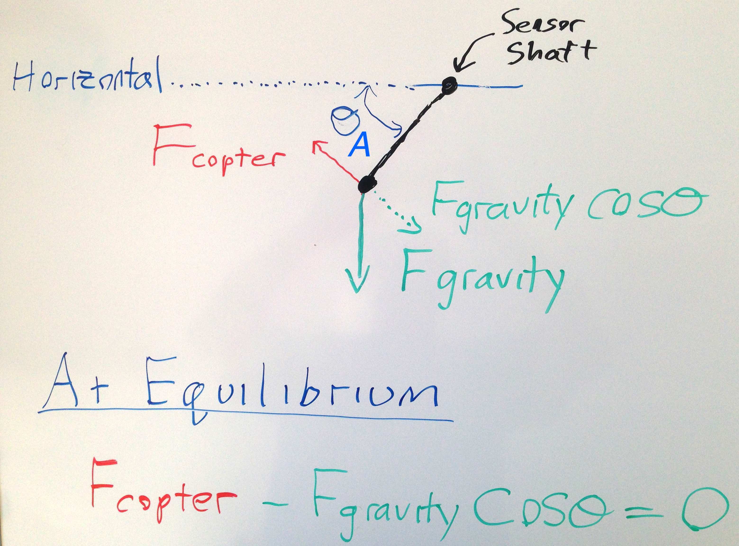
The two forces on the copter-levitated arm have different directions of action. The downward force of gravity is always pointing straight down; and the upward force produced by the spinning propeller always points in the direction of arm rotation. Whenever the arm settles at a particular rotational angle, the two forces must be in balance.

1.2.1) Let the notation begin

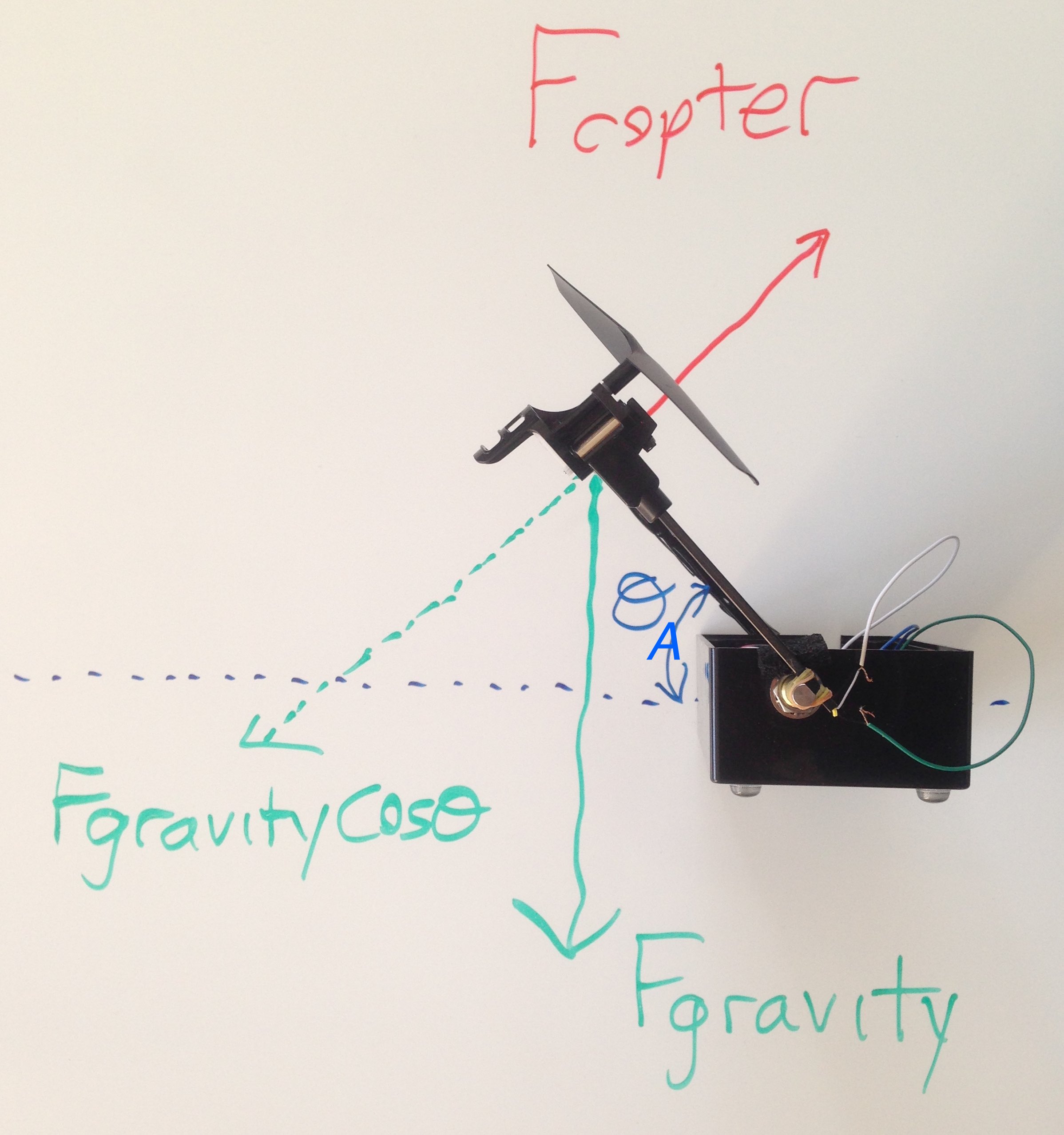
We will use \theta_A to denote the arm rotation angle, with \theta_A = 0 corresponding to a horizontal arm. The rotation forces when the arm is at an angle \theta_A from horizonal can be determined with a little trigonometry. The figure is drawn to represent, approximately, the \theta_A = -45^{\circ } case.

If the copter-levitated arm does not rotate away from its position at \theta_A = -45^{\circ } (below the horizon), we know that rotation forces on the arm must sum to zero

For the down-pointing case of \theta_A = -45^{\circ }, \cos {\theta_A } = \frac{\sqrt {2}}{2}. Balancing the forces,

and therefore f_{propeller} = \frac{\sqrt {2}}{2}f_{gravity}.

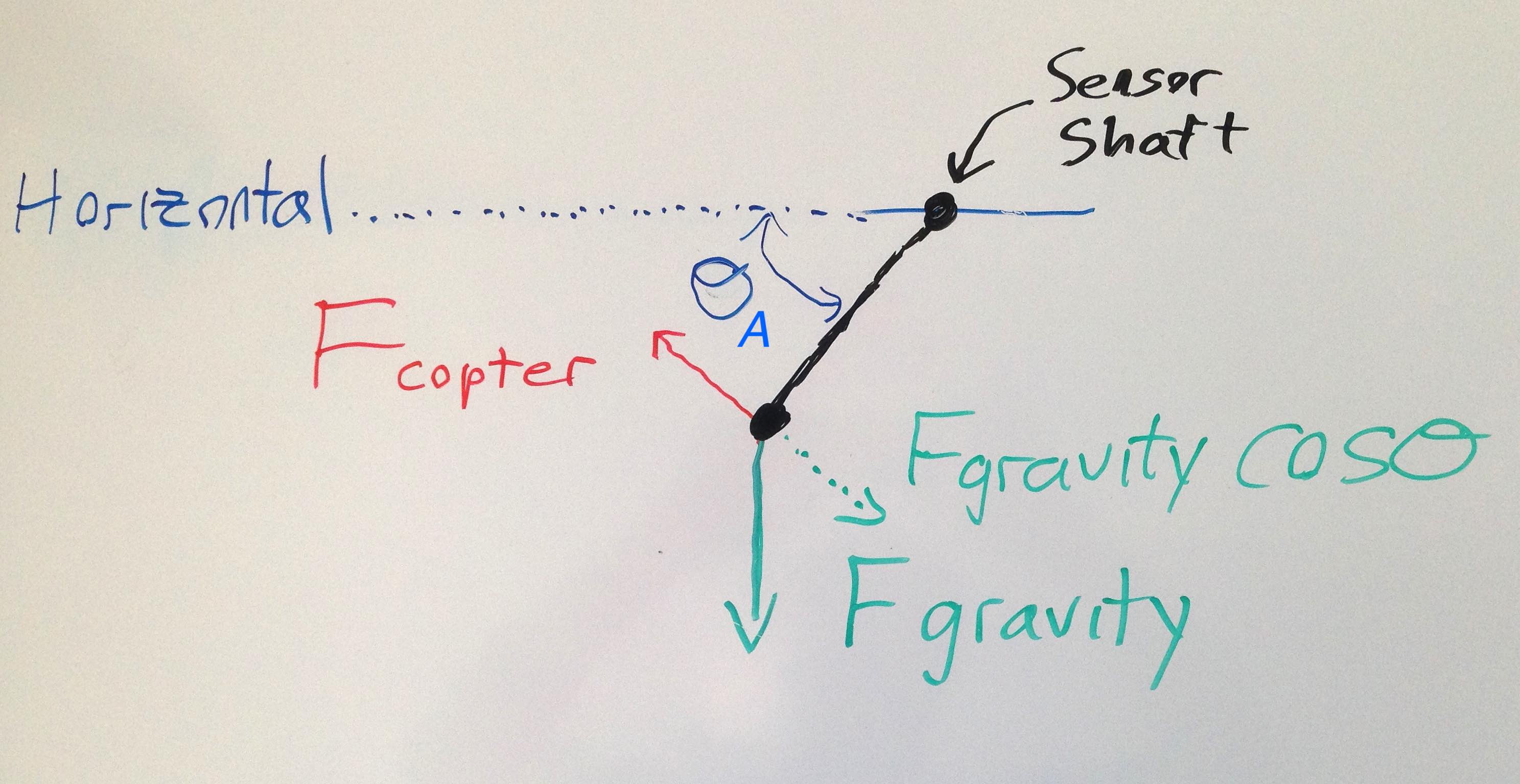
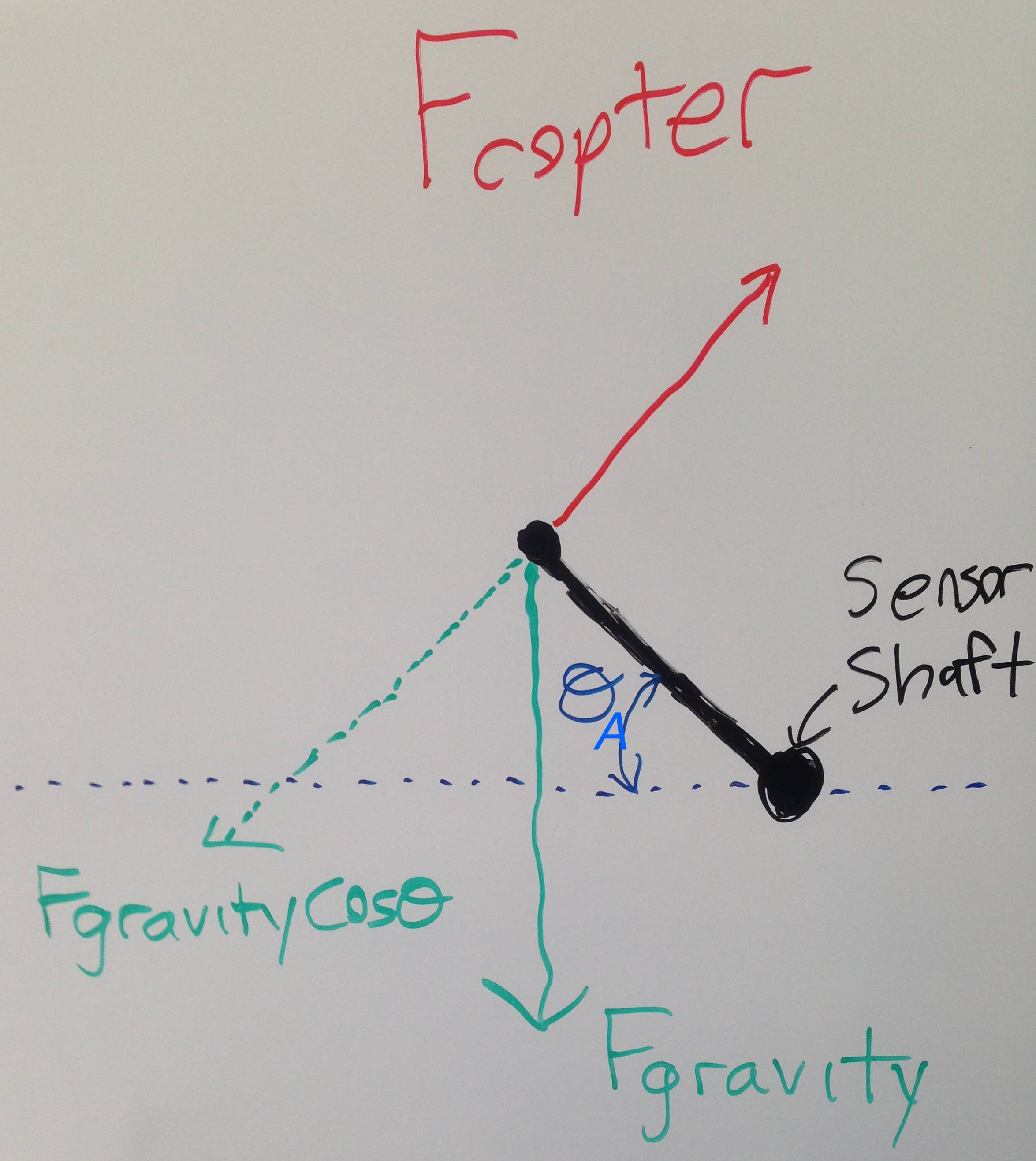
It is not possible to keep the arm 45^{\circ } above horizontal using just the direct command, but we can still analyze the propeller and gravity forces to see if they balance, as shown below.

For the case where \theta_A = +45^{\circ }, \cos {\theta_A } = \frac{\sqrt {2}}{2} just like the down-pointing case. Balancing the forces yields,

and therefore f_{propeller} = \frac{\sqrt {2}}{2} f_{gravity} in force balance.

If we compare the up-pointing and down-pointing cases, we note that the two propeller forces needed to balance gravity are identical:

Then what is the difference between the two cases? Why is it harder to position the propeller above horizontal? A more sophisticated analysis is clearly necessary.

1.3) Linearization

It seems unlikely that we will be able to use LDEs to model the copter-levitated arm problem, because \cos {\theta_A } is such a strongly nonlinear function of \theta_A over the range -90^{\circ } to 90^{\circ }. That is, there is NO proportionality constant, \gamma, such that \gamma \; \theta_A is approximately \cos {\theta_A } for all \theta_A \in [-90^{\circ },90^{\circ }] (Note that we often use the symbol \gamma when we need a generic proportionality constant, particularly when the constant must be measured by experiment. Our use of \gamma here is unrelated to its use in last week's lab). Nevertheless, we can gain some insight using LDEs, but only if we subdivide the angle interval, and use a seperate linearization in each subinterval.

First consider the down-pointing case and assume:

• the propeller force (the thrust) is always in the direction of rotation, and is given by \frac{\sqrt {2}}{2} f_{gravity}
• the arm angle only varies between -90^{\circ } and 0^{\circ }.

If we are trying to model the motion of the arm, then our primary concern is the total force in the direction of rotation,

Given our assumptions about the propeller force, the total force will be zero when \theta_A = -45^{\circ }, This suggests a linear model of the form where \theta_0 = - 45^{\circ } and \theta_a \in [-45^{\circ },45^{\circ }].

Regardless of our estimate of \gamma, when \theta_a = 0, f_{total} = 0, consistent with \theta_a = 0 corresponding to the force-balancing angle \theta_A = -45^{\circ }. One way to estimate \gamma is to use a first-order Taylor expansion of f_{total} about \theta_A = -45^{\circ }, or

The derivative of total force with respect to \theta is where the \frac{\pi}{180} is the degrees to radians conversion needed when using derivative identities. Substituting into the Taylor expansion, our linearized approximation to f_{total}(\theta_A) about \theta_0 = -45^{\circ} is

Alternatively, we could estimate \gamma by examining the total force at the extremes of \theta_a, -45^{\circ } and 45^{\circ }. When \theta_a = -45^{\circ }, the total force is just the propeller force, and is \frac{\sqrt {2}}{2} f_{gravity}. When \theta_a = 45^{\circ }, the arm is horizontal, and the total force is the propeller force minus the entire gravity force, \left(\frac{\sqrt {2}}{2} f_{gravity} - f_{gravity} \right).

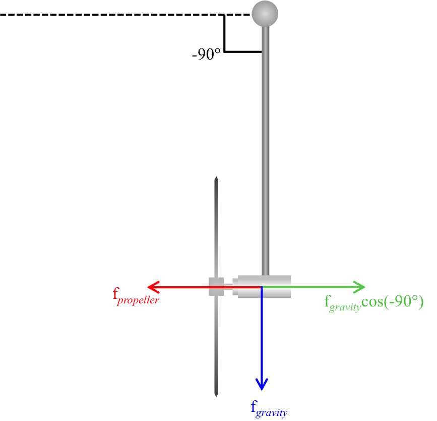
Forces when \theta_A = -90^{\circ }.

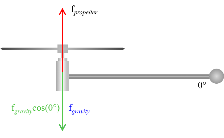
Forces when \theta_A = 0^{\circ }.

To see the above total forces relations, consider first the case of \theta_a = 45^{\circ}, or \theta_A = 0^{\circ }, and the arm is horizontal (straight out). The entire force due to gravity acts to rotate the arm (since the arm is at right angles to the direction of the force due to gravity). So the total force is the copter force (pushing up) - gravity force (pulling down), or f_{total}(0^{\circ}) = \frac{\sqrt {2}}{2} f_{gravity} - f_{gravity}.

If \theta_a = 0^{\circ } then \theta_A = -45^{\circ } and the arm is down-pointing at a negative 45^{\circ } angle. Only a part of the force due to gravity acts to rotate the arm (some of the gravity force is unsuccessfully trying to stretch the arm). So the total force trying to rotate the copter arm is copter force (rotating up) - fraction of the gravity force (rotating down), where the fraction of gravity force is \frac{\sqrt {2}}{2} or approximately 70%. Since we assumed that the gravity and propeller forces are in balance when the arm angle is \theta_A = -45^{\circ }, f_{total}(45^{\circ}) = 0.

If \theta_a = -45^{\circ } then \theta_A = -90^{\circ } and the arm is pointing straight down. None of the force due to gravity acts to rotate the arm (all of the gravity force is unsuccessfully trying to stretch the arm). So the total force trying to rotate the copter arm is propeller force, acting alone, or f_{total}(-90^{\circ}) = \frac{\sqrt {2}}{2} f_{gravity}.

From the above,

and and gives us f^{lin}_{total}(\theta_a) for the three values \theta_a=45^{\circ }, \theta_a=0, and \theta_a=-45^{\circ }.

Now lets use the approximation to the total rotating force where we assume the total force is a linear function of \theta_a. That is, we approximate the total force using a two-point difference:

remarkably close to the formula derived using a Taylor series expansion.

Comparison of force versus $ \theta_a $ for the exact case (blue line) and the linearized approximation (dots).

The f_{gravity}-normalized forces plotted in the figure above show that both linearizations (Taylor expansion or the two-point difference) are inaccurate representations of the force-\theta_a relationship at the extremes of \theta_a. Both linearized models predict forces that are not positive enough when \theta_a = -45^{\circ }, (\frac{\sqrt {2}}{2} f_{gravity} \approx -\frac{f_{gravity}}{90} (-45^{\circ}) = 0.5 f_{gravity}), and too negative when \theta_a = 45^{\circ }, (\left( \frac{\sqrt {2}}{2} - 1\right) f_{gravity} \approx -\frac{f_{gravity}}{90} (45) = -0.5 f_{gravity}). But near \theta_a = 0, the linearized approximation (particularly the Taylor series approximation) is accurate.

If you compute the two-point difference approximation for the up-pointing case, \theta_A = 45^{\circ }, what is the relationship between \theta_a and f_{total}?

2) Propeller Dynamics

Using our linear model for total force, and by following the index-shifting strategy in the Crane Mutiny example, you can derive a second-order LDE for the sequence generated by sampling \theta_a. But as we saw in lab, and you will see particularly in the second of these two examples, it is far easier to form the state-space matrix for the system, and use the fact that its eigenvalues are the natural frequencies (see notes for the week 4 lectures, for example). Then for these 2 \times 2 examples, you can compute the eigenvalues analytically.

2.1) A frictionless example

For the propeller arm example above, if we select a time between samples of 0.001 seconds (equal to the default 1000 micro-seconds between samples we typically use in lab),

where \omega_a[n-1] is (n-1)^{th} sample of the rotational velocity, and

where \alpha_a[n-1] is (n-1)^{th} sample of the rotational acceleration.

The rotational acceleration is proportional to the total force, and in our approximate model, the total force is linearly related to \theta_a, so

where \alpha_a is the arm acceleration. For this example, we will assume that the value for \gamma is \gamma = 1 or \gamma = -1. In lab, you may have already discovered that the sign of \gamma changes as you switch from the up-pointed to the down-pointed cases.

1. What are the natural frequencies for your LDEs in the up-pointing case and down-pointing cases? (NOTE: Use j=\sqrt {-1} and enter decimal representations in place of fractions wherever necessary. For example, the complex number \frac{7}{8}+\frac{1}{2}j is entered as 0.875+0.5j.)

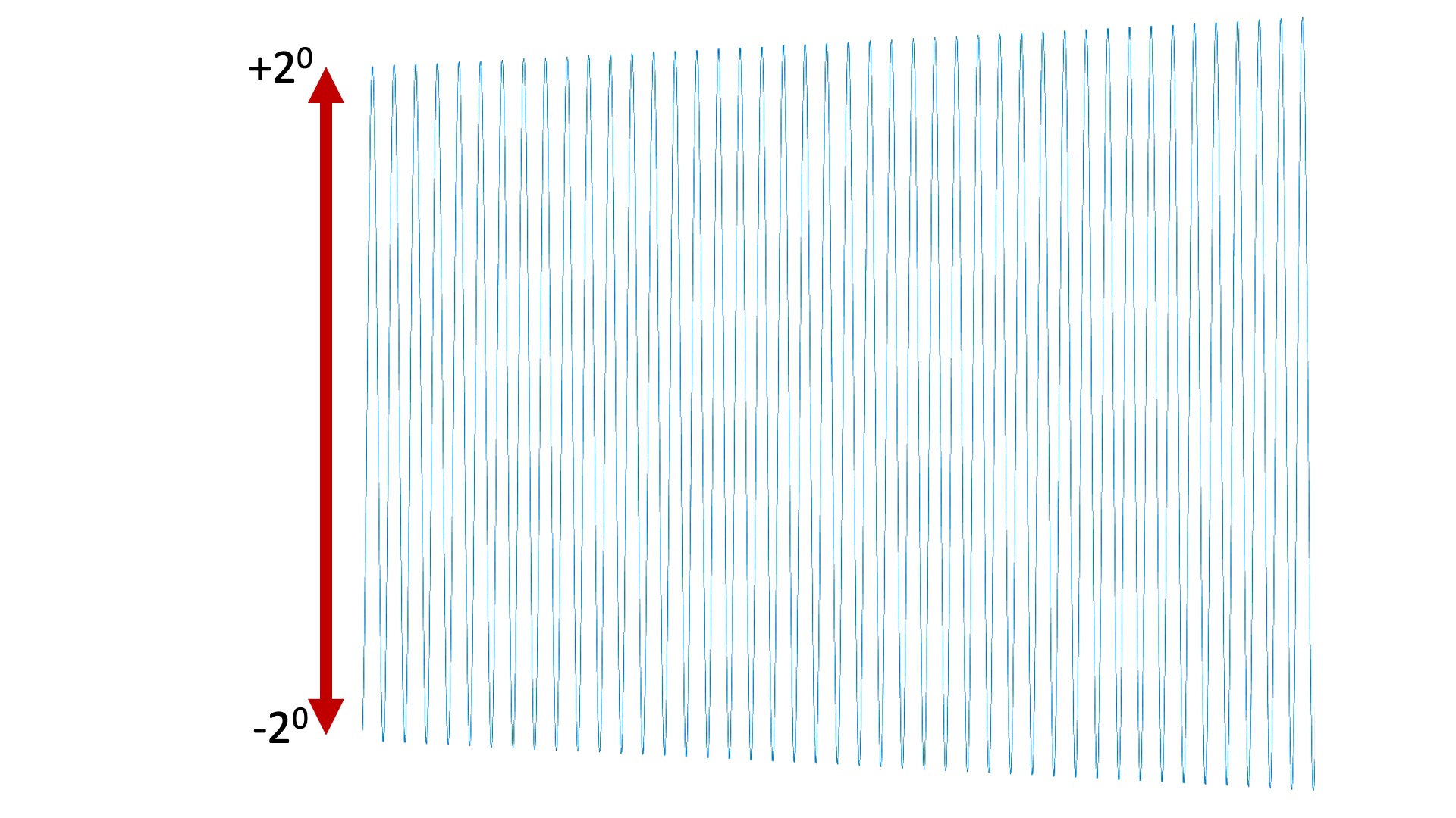
2. According to your LDE model, if the arm angle were oscillating between 2^{\circ } and -2^{\circ } about the force equilibrium point at -45^{\circ } (see figure below) in how many seconds will the arm oscillation amplitude double, that is, in how many seconds will the arm be oscillating between 4^{\circ} and -4^{\circ } about the -45^{\circ } equilibrium point.

3. Suppose we set the inital arm angle to be almost exactly 45^{\circ }, but in a few seconds we observe that the arm angle is 2^{\circ } away from 45^{\circ }. According to your LDE model, in how many more seconds will the arm be 4^{\circ } away (Hint: after the first few seconds, the response associated with the larger natural frequency will dominate).
   
   In how many seconds (after our observation) will it be 30^{\circ } away?
   

2.2) Adding Friction Example

The LDE models derived above suggest that even in the down-pointing case, if the arm angle is a few degrees away from -45^{\circ }, the arm will oscillate forever. But if you tried blowing on the propeller, to push it away from -45^{\circ }, you would have seen that the arm angle does not oscillate forever. The inconsistency is due to a modeling error, we neglected air resistance and its effect is non-negligible. So, lets try adding air resistance by approximating it as a linear friction force, and including it in our LDE models for the down-pointing and up-pointing cases.

We can add the linear friction force to the LDE model by adding a a velocity-dependent acceleration to velocity equation, as in

where \gamma \cdot \theta_a[n-1] is the acceleration due to propeller and gravity forces, and \beta \cdot \omega_a[n-1] is the deceleration due to air resistance.

What is a reasonable value for \beta? The frictional force is always fighting against direction of motion so \beta must be negative. For this model, we will try using \beta = -1, and see if the model better matches observations.

1. What are the natural frequencies for your LDEs in the up-pointing case and down-pointing cases

2. Suppose you puff on the propeller and notice that its peak displacement from -45^{\circ } is 2^{\circ }. According to your LDE model with friction, to within 50%, what is the maximum displacement from -45^{\circ } you will see if you wait 5 seconds after the peak? What if you wait 10 seconds? (Hint: it is easiest if you consider magnitudes).

3. Suppose we set the inital arm angle to be almost exactly 45^{\circ }, but in a few seconds we observe that the arm angle is 2^{\circ } away from 45^{\circ }. According to your LDE model with friction, what will the arm angle displacement be after 5 more seconds? After 10 more seconds (Hint: after the first few seconds, the response associated with the larger natural frequency will dominate)? Another Hint: You'll need a lot of significant digits - at least to the hundred-thousandths - in your lambda for this calculation. If you're using MATLAB use 'format LONG' in your command window to get more significant digits.