Linear Differential Equations and Complex Exponentials

The questions below are due on Thursday March 14, 2024; 10:30:00 PM.

You are not logged in.
Please Log In for full access to the web site.
Note that this link will take you to an external site (https://shimmer.mit.edu) to authenticate, and then you will be redirected back to this page.

(Adapted from notes by T.F. Weiss)

1) Outline

To outline what follows:

A summary of the transition from DT to CT
Sources of linear differential equations
Homogeneous solution --- exponential solution, natural frequencies
Particular solution --- system function, poles and zeros
Total solution --- matching initial conditions.
The system function, H(s), and its use in block diagrams.

2) DT to CT Summary

We started in discrete time, using linear difference equations (LDEs) to model motor and arm behavior. In continuous time, we replace difference equations with differential equations, replace shifts in index with derivatives in time, and replace integer index n with real scalar t. Despite the changes, we we can still refer to linear DIFFERENTIAL equations as LDEs.

In discrete-time, when our system model was a set of difference equations, we packed those equations into a state-space description, and found the system's natural frequencies by computing the eigenvalues of its associated state-space matrix \mathbf{A}. In CT, we will approach the problem differently (for reasons that will be clear soon) and compute natural frequencies by substituting solutions based on assuming a parameterized form, e.g. u(t) = U e^{st}, which we plug into the LDE to determine parameters.

The approach relies on a key property, that derivatives of an exponential function are related by a scale factor. For example,

if \;\; u(t) = U e^{st},\;\; then\;\; \frac{d}{dt} u(t) = U se^{st} = s u(t).

In continuous time, the general form for an LDE with input time function u and output time function y is

\sum_{l=0}^L a_l \frac{d^l y(t)}{dt^l} = \sum_{\tilde{l}=0}^{\tilde{L}} b_{\tilde{l}} \frac{d^{\tilde{l}} u(t)}{dt^{\tilde{l}}},

Notice the equation involves u and its derivatives, which are on the right side because they are "known", and involves y and is derivatives, are all on the left of the equality, because none are "known".

Plugging in the assumed form u(t) = U e^{st} and y(t) = Y e^{st},

\left(\sum_{l=0}^L a_l s^{l} \right) Y e^{st} = \left( \sum_{\tilde{l}=0}^{\tilde{L}} b_{\tilde{l}} \right) U e^{st}.

Cancelling the e^{st} and dividing by the left-side polynomial, Y can be related to U with

Y = H(s) U,

were H(s) is referred to as a transfer function (for reasons we make clear below) and is a ratio of polynomials in s,

H(s) = \frac{n(s)}{d(s)} = \frac{\sum_{\tilde{l}=0}^{\tilde{L}} b_{\tilde{l}} s^{\tilde{l}}}{\sum_{l=0}^L a_l s^{l}}.

The CT natural frequencies are the values of s for which

\left(\sum_{l=0}^L a_l s^{l} \right) = 0,

or equivalently, the roots of the denominator polynomial, d(s).

2.1) Finding y(t) given u(t)

Given an input u(t) = U e^{s_0 t}, we can find a particular solution y_p(t) = Y e^{s_0 t}, then

\left(\sum_{l=0}^L a_l s_0^{l} \right) Y e^{s_0t} = \left( \sum_{\tilde{l}=0}^{\tilde{L}} b_{\tilde{l}s^{\tilde{l}}} \right) U e^{s_0t},

Y = H(s)|_{s = s_0} U.

To match the initial condition, we can add a weighted combination of of natural frequency exponentials to the particular solution, as in

y(t) = \sum_{l=1}^{L} A_{l} e^{\lambda_l t} + H(s)|_{s = s_0} U e^{s_0 t},

where the \lambda_i's are the system's natural frequencies and are equal to the roots of H(s)'s denominator polynomial. The A_{l}'s are determined by matching L values of y(t) and its derivatives, usual at t=0 (initial values), e.g.

\frac{d^l}{dt^l} y(t)|_{t=0} \;\;for \;\; l \in \{0,1,,..,L-1\}.

2.2) Natural Frequencies and Stability.

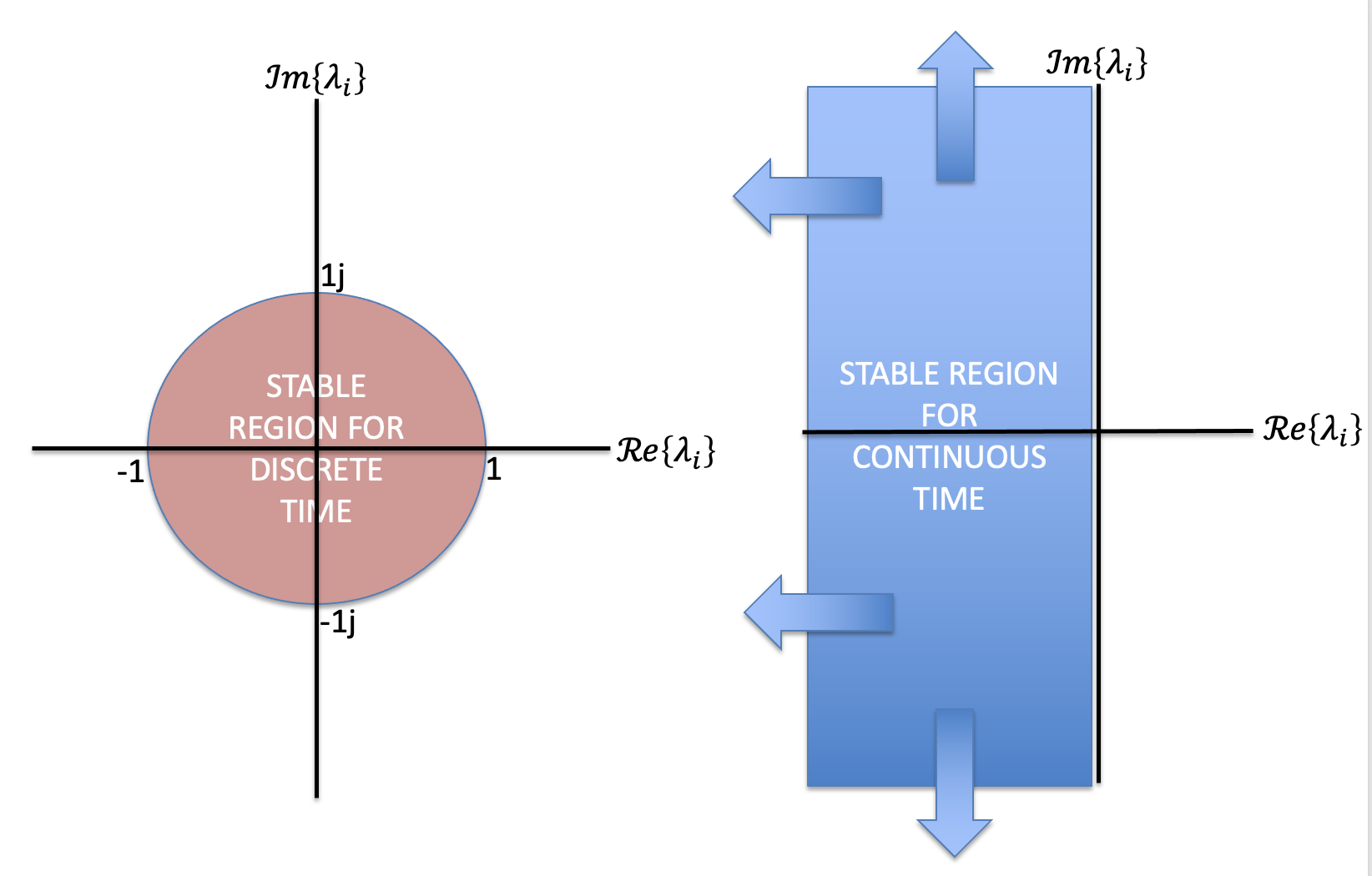
For systems described by difference equations in DT or differential equations in CT, determining natural frequencies involves finding the (possibly) complex roots of the system's characteristic polynomial. Finding DT and CT natural frequencies may lead to similar computational problems (polynomial root-finding), but their impact onn behavior is definitely NOT similar.

Of particular concern are natural frequencies that correspond to homogenous solutions that are growing (unstable), or decaying (stable). In discrete time, if all of a difference equation's natural frequencies are inside the unit circle, |\lambda_i| < 1 for all i, then since \lambda_i^n decays to zero for alli, the system is stable. In the continuous time case, if all the natural frequencies are in the left-half plane, \Re{(\lambda_i)} < 0 for all i, then e^{\lambda_i t} decays to zero for all i, and the CT system is stable.

To examine the behavior due to CT natural frequencies more closely, consider that a complex number \lambda can be written in real-imaginary or magnitude-angle form. That is,

\lambda = a+bj = Me^{j \theta} = M \; (\cos{\theta} + j\sin{\theta})

where a and b are real scalars, M = \sqrt{a^2 + b^2} and \theta = \arctan{\frac{b}{a}} are the complex number's magnitude and angle.

In discrete time, natural frequencies are related to difference equation solutions through the power function. So if \lambda is a discrete-time system's natural frequency, then we are concerned with

\lambda^n = M^n e^{j \theta n} = M^n \left(\cos{\theta n} + j\sin{\theta n}\right).

If M > 1 then lim_{n\rightarrow \infty} |\lambda^n| \rightarrow \infty and we say the system is unstable.

In continuous time, natural frequencies are related to differential equation solutions through the exponential function. So if \lambda is a differential equation's natural frequency, then we are concerned with

e^{\lambda t} = e^{(\sigma+j\omega)t} = e^{\sigma t} e^{j\omega t} = e^{\sigma t} \left(\cos{\omega t} + j\sin{\omega t}\right).

If the real part of \lambda is greater than zero, \Re{(\lambda)} = \sigma > 0, then |e^{\lambda t}| = e^{\sigma t} \rightarrow \infty and the system is unstable.

Regions of the complex plane corresponding to decaying natural frequencies (Region of stable natural frequencies). On the left, the region of stable natural frequencies for DT is the unit disk (|\lambda_i| < 1), and on the right, the region of stable natural frequencies for CT is the left-half plane (\Re{(\lambda)} < 0 ).

3) Linear Differential Equations Examples

3.1) An electrical network

Kirchoff's current law yields

i(t) = i_C(t) + i_R(t) + i_L(t) .

The constitutive relations for each element yield

i_C = C {dv(t) \over dt}, \hspace{0.15in} i_R(t) = {v(t) \over R}, \hspace{0.15in} i_L(t) = {1 \over L}\int_{-\infty}^t v(\tau)\, d\tau .

Combining KCL and the constitutive relations yields

{di(t) \over dt} = C {d^2v(t) \over dt^2} + {1 \over R} {dv(t) \over dt} + {v(t) \over L}.

3.2) Mechanical system example

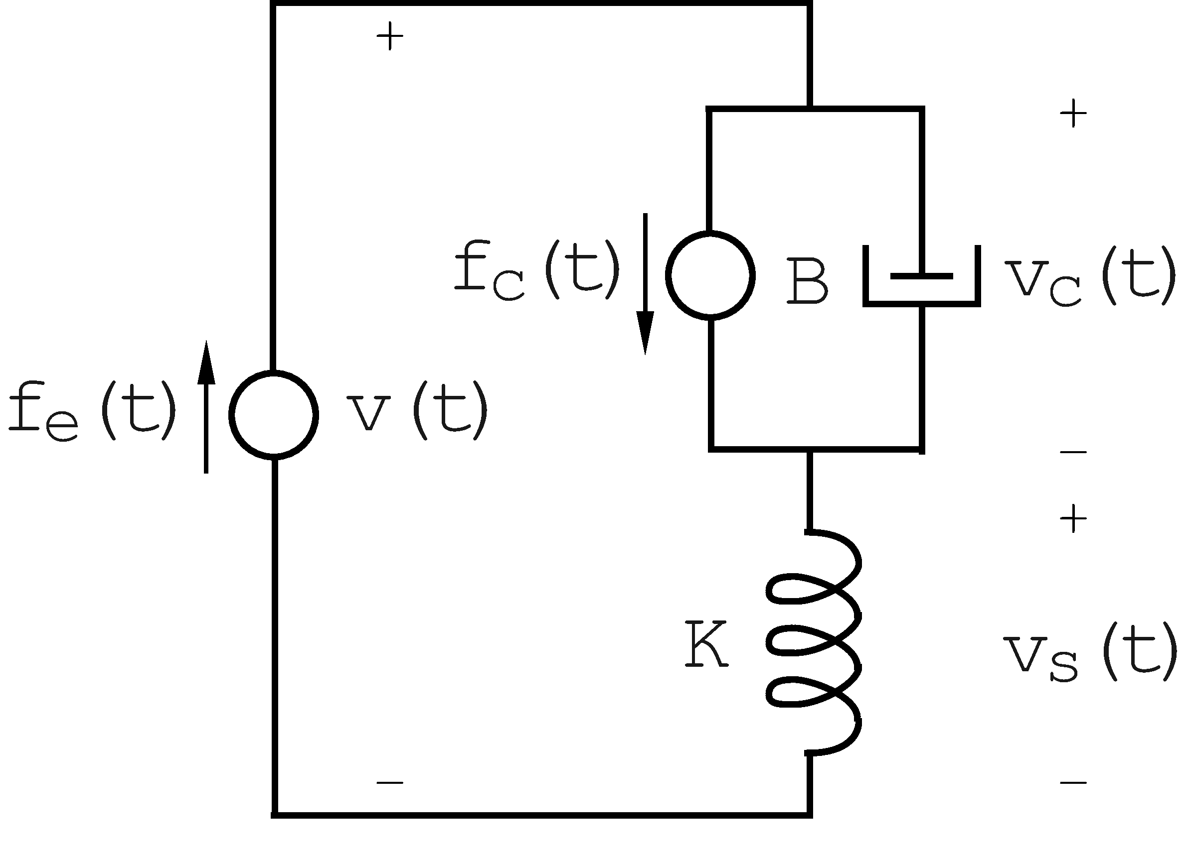
The simplest possible model of a muscle (the linearized Hill model) consists of the mechanical network shown below, in which the rate of change of the length of the muscle, v(t), is related to the the external force on the muscle f_e(t).

A spring-mass-dashpot model of a muscle, f_c is the internal force generated by the muscle, K is its stiffness and B is its damping.

The muscle velocity can be expressed as

v(t) = v_c(t) + v_s(t) .

\end{slide} \begin{slide} \bottomlevel{Mechanical system, cont'd} Combining the muscle velocity equation with the constitutive laws for the elements yields

v(t) = {f_e(t) - f_c(t) \over B} + {1 \over K} {df_e(t) \over dt} .

3.3) First-order chemical kinetics

A reversible,first-order chemical reaction can be represented as follows

\mathrm{R} \xrightleftharpoons[\alpha]{\beta} \mathrm{P}

where R is the reactant and P is the product. The concentrations of reactant and product are c_R(t) and c_P(t). In such a reaction, the rate equation is given by

-{dc_R(t) \over dt} = \alpha c_R(t) - \beta c_P(t) .

If reactant and product are conserved,

c_R(t) + c_P(t) = C.

After substitution, we obtain

{dc_R(t) \over dt} + (\alpha + \beta) c_R(t) = \beta C .

3.4) General Form of an LDE

For many "lumped" physical systems the input, u(t), can be related to the output, y(t), by an nth order differential equation of the form

\sum_{l=0}^L a_l \frac{d^l y(t)}{dt^l} = \sum_{\tilde{l}=0}^{\tilde{L}} b_{\tilde{l}} \frac{d^{\tilde{l}} u(t)}{dt^{\tilde{l}}},

where that high order differential equation system may be the result of composing several first-order differential equations, just like we saw in the case of difference equations.

4) LDE Solutions

When we studied difference equations describing discrete-time systems, we focused on computing solutions for two cases:

The Zero Input, or Homogenous, case with non-zero initial conditions,
The Step Response case, where the input is the time-shifted unit step and the initial conditions are zero.

When it comes to differential equations describing continuous-time systems, we will be interested in more than just homogenous solutions and step responses, we will also be interested in the system's response to sinusoidal inputs over a range of frequencies. These frequency responses will help us better characterize our systems, and will also help us design CT control systems, as we will see over the next few weeks.

4.1) Homogeneous Solutions

Let the homogeneous solution be y_h(t), then the homogeneous equation is

\sum_{l=0}^L a_l {d^l y_h(t) \over dt^l} = 0 .

To solve this equation we assume a solution of the form

y_h(t) = A e^{s t} .

Since

{d^n y_h(t) \over dt^n} = A s^n e^{s t} ,

we have

\sum_{l=0}^L a_l A \lambda^l e^{s t} = \left(\sum_{l=0}^L a_l s^n\right) A e^{s t} = 0 .

Since we are only interested in non-trivial solutions, we can assume A \ne 0, ensuring that y_h(t) = A e^{s t} \ne 0 for all t > 0. Dividing the above equation by A e^{s t} results is the characteristic polynomial for the LDE,

\left(\sum_{l=0}^L a_l s^l\right) = 0 .

This polynomial of order L has L roots,

\{ \lambda_1,...,\lambda_l \}

which can be exposed by writing the polynomial in factored form

\prod_{l=1}^L \left(s - \lambda_l\right) = 0.

The roots of the characteristic polynomial

\{\lambda_1,\lambda_2,\ldots\lambda_L\}

are the natural frequencies . These are frequencies for which there is an output in the absence of an input. For example, imagine striking a (somewhat idealized) tuning fork. After the tuning fork has been struck there is no further input, but the tuning fork keeps vibrating --- at its natural frequencies.

Do not be confused by the tuning fork example, the vibration frequency is NOT a natural frequency. Since the fork's vibration eventually dies away, the natural frequencies associated with the vibration are a pair of complex numbers. Both have the same real part, a negative number that indicates the decay rate, and the same magnitude of the imaginary part (negative in one and positive in the other), which indicates the vibration frequency.

If the natural frequencies are distinct, i.e., if \lambda_i NOT equal to \lambda_k for all i not equal to k, then the most general homogeneous solution has the form

y_h(t) = \sum_{l=1}^L A_l e^{\lambda_l t} .

4.2) Circuit Natural Frequency Examples

The differential equation relating v(t) to i(t) is

{di(t) \over dt} = C {d^2v(t) \over dt^2} + {1 \over R} {dv(t) \over dt} + {v(t) \over L} .

The characteristic polynomial is

\lambda^2 + {1 \over RC} \lambda + {1 \over LC} = 0 .

The roots of this quadratic characteristic polynomial, the natural frequencies, are

\lambda_{1,2} = - {1 \over 2RC} \pm \sqrt{\left({1 \over 2RC}\right)^2 - {1 \over LC}} .

The locus of natural frequencies is plotted for L=C=1 with R increasing in the directions of the arrows. Note the natural frequencies are in the left-half plane for all values of R>0 . As R\rightarrow \infty , the natural frequencies approach the imaginary axis. What is the physical significance of this behavior?

4.3) Exponential Input Response

Now we need to find a particular solution to the differential equation

\sum_{l=0}^L a_l {d^l y_p(t) \over dt^l} = \sum_{\tilde{l}=0}^{\tilde{L}} b_{\tilde{l}} {d^{\tilde{l}} u(t) \over dt^{\tilde{l}}} .

assuming zero initial conditions and an exponential input. More specifically,

{d^l y_p(t) \over dt^l}|_{t=0} = 0 \;\;\; for\; all \; l \in [0,L-1],

and u(t) is given by

u(t) = Ue^{s_0 t}, \; \; \; for \; all \; t > 0,

where U and s_0 are general complex scalars.

If we assume s_0 is NOT equal one of the natural frequencies, then

y_p(t) = Ye^{s_0 t} ,

will satisfy the differential equation with non-zero input, and we can solve for Y.

Substitution for both u(t) and y(t) in the differential equation yields, after factoring,

\left(\sum_{l=0}^L a_l s_0^l \right) Y e^{s_0t} = \left(\sum_{\tilde{l}=0}^{\tilde{L}} b_{\tilde{l}} s_0^{\tilde{l}} \right) U e^{s_0 t}.

We can again divide by e^{s_0 t}, and solve for Y given U.

The relationship between the complex scalar Y and the complex scalar U depends on the frequency of the input, s_0, and has the form

Y = H(s)|_{s=s_0} U ,

where

H(s)|_{s=s_0} = {\sum_{\tilde{l}=0}^{\tilde{L}} b_{\tilde{l}} s_0^{\tilde{l}} \over \sum_{l=0}^L a_l s_0^l} .

4.4) The Total solution

The general solution to the LDE, given the input Ue^{s_0 t}, has a particularly simple form if we assume that the natural and input frequencies are unique,

\lambda_1 \ne \lambda_2 , \ne....\ne \lambda_L \ne s_0.

Under this modest assumption,

y(t) = \underbrace{\sum_{l=1}^L A_l e^{\lambda_l t}}_{homogeneous} + \underbrace{H(s)|_{s=s_0}Ue^{s_0t}\rule[-1em]{0em}{2em}}_{particular}.

Note that to completely compute the solution, we would need to determine the L coefficients

\{A_1,A_2,\ldots,A_L\}.

While the L coefficients can be determined from any L values of y(t) and its derivatives, it is most common to determine them from the t = 0 values for y(t) and {d^l y(t) \over dt^l} , l \in {1,...,(L-1)}.

The total solution can also be computed using the unilateral Laplace transform, but as we will see in the following weeks, we will have little reason to investigate the impact of specific initial conditions.

5) The System Function

H(s) = {\sum_{\tilde{l}=0}^{\tilde{L}} b_{\tilde{l}} s^{\tilde{l}} \over \sum_{l=0}^L a_l s^l} .

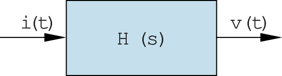
is called the system or transfer function,
is a rational function in s,
is a skeleton of the differential equation,
characterizes the relation between u(t) and y(t).

5.1) Reconstructing the LDE from H(s)

Suppose

H(s) = {s \over s+1} ,

what is the differential equation that relates the output y(t) to the input u(t)?

Step to reverse the steps used to compute H(s) by cross-multiplying

Ye^{st} = H(s) Ue^{st} ,

by the denominator polynomial of H(s), to get

(s+1)Ye^{st} = sUe^{st},

sYe^{st} + Ye^{st} = sUe^{st}.

Then taking one more reverse step, we obtain the differential equation

{dy(t) \over dt} + y(t) = {du(t) \over dt} .

In general, H(s) can be expressed in factored form as follows

H(s) = K \frac{{\prod_{\tilde{l}=1}^{\tilde{L}}} (s - s_{z_{\tilde{l}}})} {\prod_{l=1}^L (s - s_{p_l})},

where K = \frac{b_{\tilde{L}}}{a_L}.

\{s_{z_1},s_{z_2},\ldots s_{z_M}\} are the roots of the numerator polynomial and are called zeros of H(s) because these are the values of s for which H(s)=0.
\{s_{p_1},s_{p_2},\ldots s_{p_N}\} are the roots of the denominator polynomial and are called poles of H(s) because these are the values of s for which H(s)=\infty.

5.2) Poles are the natural frequencies

Note that poles of H(s) are the natural frequencies of the system. Recall that natural frequencies are given by the roots of the polynomial,

\left(\sum_{l=0}^L a_l \lambda^l\right) = 0,

which are also the roots of the denominator polynomial of H(s)

\left(\sum_{l=0}^L a_l s^l\right) = 0 .

Both originate from the left-hand side of the differential equation

\sum_{l=0}^L a_l {d^l y(t) \over dt^l} .

5.3) Pole-zero diagram

The system function, H(s), completely characterizes the differential equation, and H(s) is characterized by the location of L poles, \tilde{L} zeros, and an overall scale factor K. We can characterize how H(s) changes with s using a pole-zero diagram, a plot of the locations of poles and zeros in the complex-s plane. The ordinant is j\Im\{s\} = j\omega and the abscissa is \Re\{s\} = \sigma where

s = \sigma + j\omega .

5.4) Example --- system function of a circuit

The differential equation relating v(t) to i(t) is

{di(t) \over dt} = C \left( {d^2v(t) \over dt^2} + {1 \over RC} {dv(t) \over dt} + {v(t) \over LC}\right) .

The particular solution is obtained from

sI = C\left(s^2 + {1 \over RC} s + {1 \over LC}\right)V .

With v(t) as the output and i(t) as the input, the system function of the RLC network is

H(s) = {V \over I} = {1 \over C}\left({s \over s^2 + {1 \over RC} s + {1 \over LC}}\right).

5.5) A Small Example

Given the system function

H(s) = {Y \over U} = {s+2 \over (s+3)(s+4)},

what are the natural frequencies of the system? What is the differential equation that relates u(t) and y(t)?

Solution

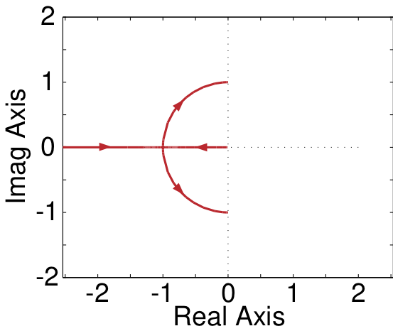
The natural frequencies of the system are the poles of the system function and are -3 and -4.

The differential equation can be obtained by cross multiplying and multiplying by e^{st} to obtain

(s+3)(s+4)Ye^{st} = (s+2)Ue^{st} ,

(s^2+7s+12)Ye^{st} = (s+2)Ue^{st} ,

so that

{d^2 y(t) \over dt^2} + 7 {dy(t) \over dt} + 12 y(t) = {du(t) \over dt} + 2 u(t) .

6) Key Points

6.1) Circuit Examples

An example structural description (e.g. a circuit):

has an equivalent functional description:

where

H(s) = {V \over I} = {1 \over C}\left({s \over s^2 + {1 \over RC} s + {1 \over LC}}\right).

is the circuit's transfer function from current in to voltage out.

6.2) The importance of System/Transfer Functions.

There are many ways to compute LDE natural frequencies, and to compute LDE solutions given an input. If that is all we were doing, we would not need transfer functions. But suppose your system is a composition of smaller subsystems, in series or parallel, possibly surrounded by feedback? Given the transfer function description of each subsystem, you can easily compute the overall system function, a computation that will only involve forming products, sums and ratios of the subsystem transfer functions.

In the figure below, we note some examples of composition: parallel sum, sequential application, and feedback.

Creating more complex systems from simpler ones, by parallel application and summing (top row), sequential application (middle row), or a combination of the two in concert with feedback, bottom row.

Since transfer functions are rational functions, computing products and sums is a bit more complicated that suggested by the above figure. Multiplying transfer functions involves forming products of numerator and denominator polynomials, maybe not as much fun as it sounds. Nevertheless, once you find H(s) for your composite system, you can compute poles, determine input responses, and even generate a whole-system differential equations.

7) Practice exercises.

Let's revist the simple model for the propeller arm, and redo it in CT. But before beginning, we note that we often prefer to write CT block diagrams and system descriptions in terms of integrals rather than derivatives. So for the propeller example, we could write the CT version of the arm equations: the time derivative of position is velocity and the time derivative of velocity is acceleration. Instead, we prefer to think of position as the time integral of velocity, and velocity the time integral of acceleration.

From the perspective of computing transfer functions, we can use either approach. Suppose, for example, that

\frac{d}{dt} y(t) = u(t),

which we can write as an integral,

y(t) = \int u(\tau) d\tau.

Assuming u(t) = U e^{st} and y(t) = Ye^{st}, we get

Y = H(s) U = \frac{1}{s} U,

regardless of which form we write the equations.

Consider the block diagram below, showing both the time and transfer function representation of the propeller arm. In the diagram, \alpha_a(t) is the arm rotational acceleration, \omega_a(t) is the arm rotational velocity, \theta_a(t) is the arm rotation angle, \gamma is the linearized coefficent for the angle-dependent gravity-related force, \beta an air resistance coefficient, and c(t) is a command input.

The integrator-adder-gain block diagram for the propeller arm, top, and its block diagram for computing H(s) , bottom.

The equations for the propeller arm, using integrals and then transfer functions are:

\omega_a(t) = \int \alpha_a(\tau) d\tau, \;\;or\;\; \Omega_a = \frac{1}{s} \Alpha_a,

\theta_a(t) = \int \omega_a(\tau) d\tau, \;\;or\;\; \Theta_a = \frac{1}{s} \Omega_a,

\alpha_a(t)= \gamma \theta_a(t) - \beta \omega_a(t) + c(t) \;\;or\;\; \Alpha_a = \gamma \Theta_a - \beta \Omega_a + C.

In answering the questions below, use a python expressions. Please use B for \beta, G for \gamma and s for the s. For example, \frac{\gamma}{s^3+ \beta} should be written as 'G/(s**3 + B)'.

Give an expression for transfer function relating the input command to angle, assuming \gamma =\beta = 0,

\Theta_a = H_{C2\Theta} (s) C

H_C2Th (G=B=0) =

Give an expression for transfer function relating the input command to angle, now assuming a nonzero \gamma, but \beta = 0

H_C2Th (B=0, use G for Gamma) =

Give an expression for transfer function relating the input command to angle, now assuming a nonzero \beta, but \gamma = 0

H_C2Th (G=0, use B for Beta) =

Give an expression for transfer function relating the input command to angle, now assuming a nonzero \beta and nonzero \gamma

H_C2Th(G and B nonzero, use G for Gamma, B for Beta) =

Give an expression for transfer function relating the input command to rotational velocity \Omega_a, assuming \gamma and \beta are both nonzero.

H_C2Omega = (B for Beta, G for Gamma)

Suppose the natural frequencies of the system are 4j and -4j? What are the values of \gamma and \beta. Watch the sign of \gamma!!

Beta if nat freqs +/- 4j:

Gamma if nat freqs +/- 4j:

Suppose the natural frequencies of the system are 2+4j and 2-4j? What are the values of \gamma and \beta.

Beta if nat freqs 2+/- 4j:

Gamma if nat freqs 2+/- 4j:

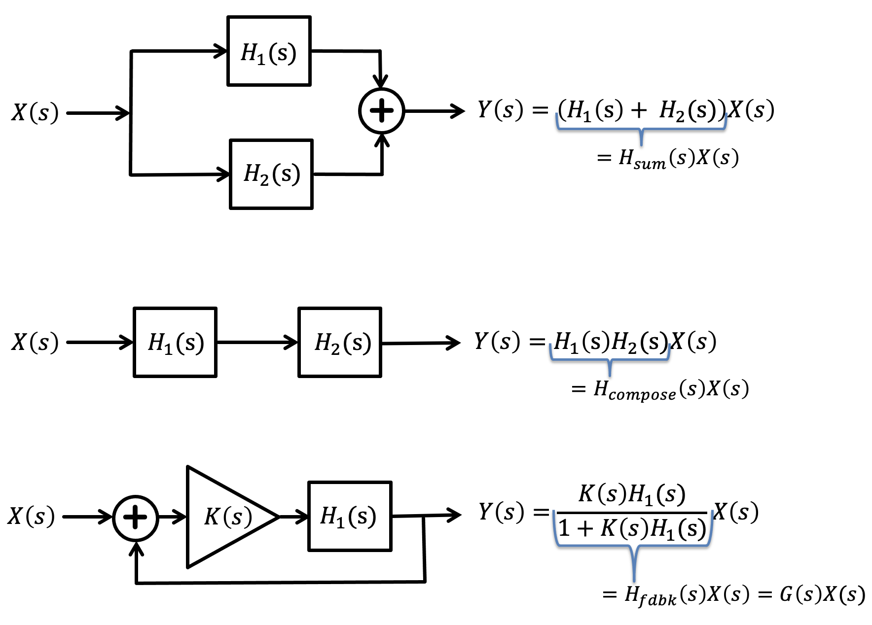
Below are five plots of \theta(t) in response to a step change in c(t) (c(t) = 0, t < 0, c(t) = 1, t \ge 0). The five plots are numbered, and below the plots are five lettered \beta, \gamma pairs which we are asking you to match to the plots. For each of the five plots, determine the letter of the \beta, \gamma pair to make a five-letter "word" (note that "not in this list" is an option you will need, so your word should have an "N" in it!). Then give your five-letter as the answer to this question.

You should be able to solve this without resorting to computer plots. Think about the relationship between \beta, \gamma, and the pair of natural frequencies.

1: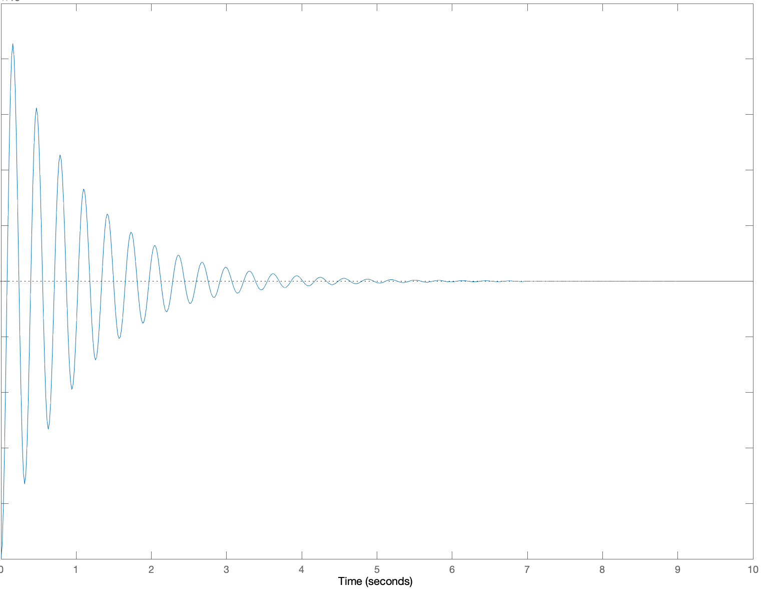

2: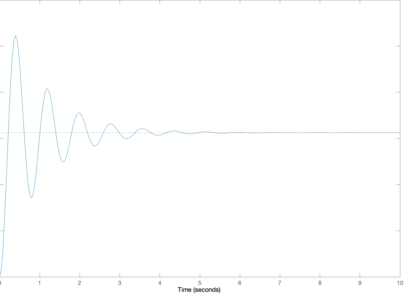

3: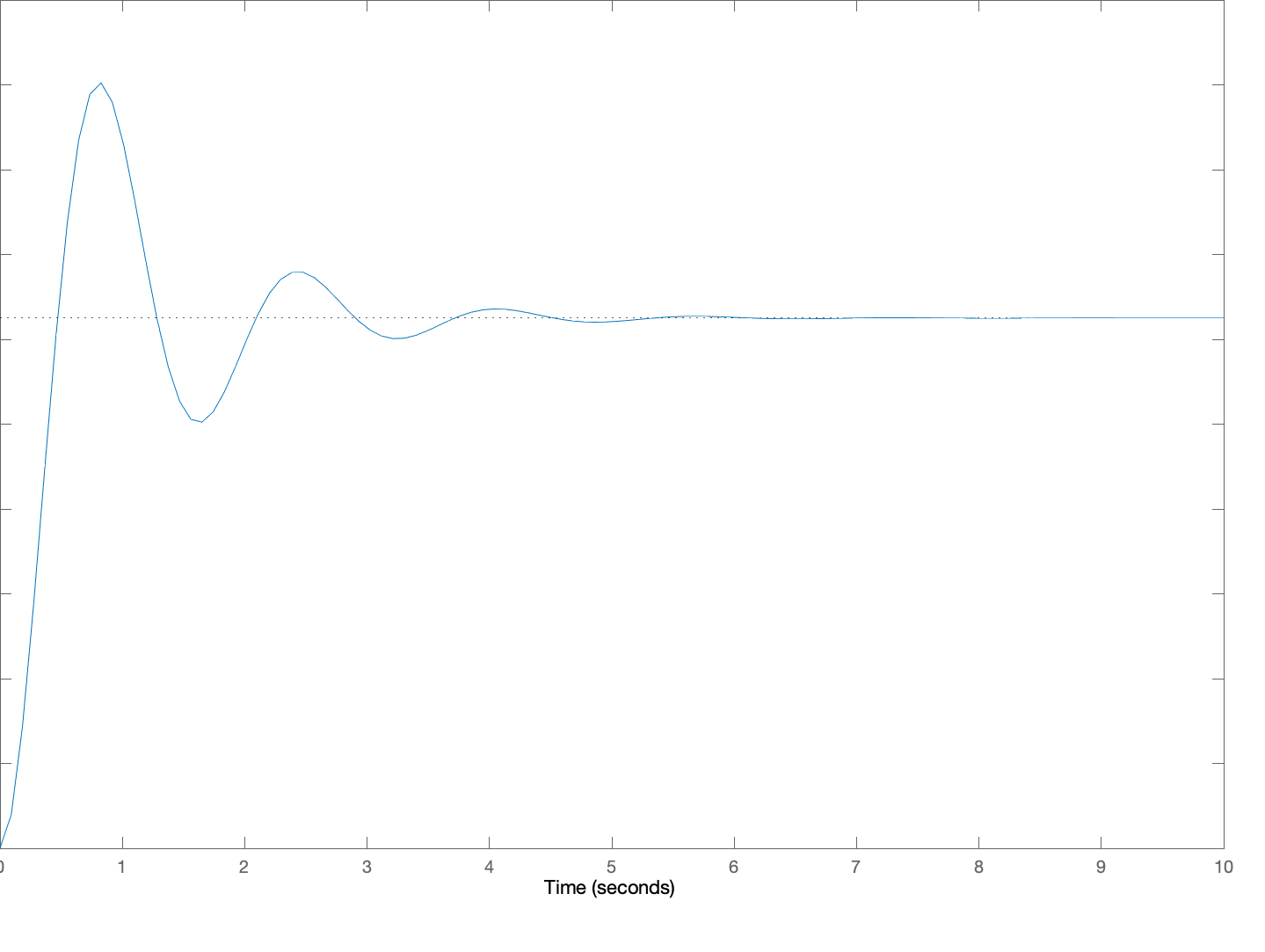

4: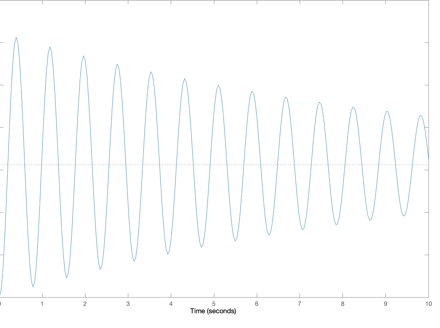

5:

Create a five-letter "word" by matching each of the above plots to a letter associated with its \beta and \gamma pair. For example, if you think plot 1 goes with A, \beta= 0.2\;\;\ \gamma = 16, plot 2 goes with B, plot 3 with C, plot 4 with D and plot 5 is not in the list, enter 'ABCDN'. Be sure to use CAPITAL letters.

A: \beta= 0.2\;\;\ \gamma = -16

B: \beta= 0.2\;\;\ \gamma = -64

C: \beta= 2\;\;\ \gamma = -16

D: \beta= 2\;\;\ \gamma = -64

E: \beta= 2\;\;\ \gamma = -96

N: Not in this list

Give a set of five letters (eg ACBND)