Closing the Loop around K(s)H(s)

The questions below are due on Thursday March 14, 2024; 10:30:00 PM.

You are not logged in.
Please Log In for full access to the web site.
Note that this link will take you to an external site (https://shimmer.mit.edu) to authenticate, and then you will be redirected back to this page.

Are Poles Sufficient?

1) A quick reminder

For the systems we consider in this class, ones accurately-modeled by sets of linear differential equations, the system (or transfer) function completely characterizes the system. And in general, H(s) can be expressed in factored form,

H(s) = \frac{n_h(s)}{d_h(s)} = K \frac{{\prod_{\tilde{l}=1}^{\tilde{L}}} (s - s_{z_{\tilde{l}}})} {\prod_{l=1}^L (s - s_{p_l})},

where K can be determined by matching to H(s) at some value, usually the limit as s \rightarrow 0 or s \rightarrow \infty.

Here, \{s_{z_1},s_{z_2},\ldots s_{z_M}\} are the roots of the numerator polynomial and are called zeros of H(s) because these are the values of s for which H(s)=0 and \{s_{p_1},s_{p_2},\ldots s_{p_N}\} are the roots of the denominator polynomial and are called poles of H(s) because these are the values of s for which H(s)=\infty.

If we have a feedback system with primary input y_{desired}(t), and the input to the "plant" described by H(s) is

K_0 (y_{desired} (t) - y(t))

where y(t) is the output of the plant, then the transfer function from Y_{desired} to Y is

G(s) = \frac{K_0 H(s)}{1 + K_0 H(s)}

or in terms of polynomials,

G(s) = \frac{n_g(s)}{d_g(s)} = \frac{K_0 n_h(s)}{d_{h}(s) + K_0 n_{h}(s)}.

The above formula suggests that as K_0 grows from a small gain to a large one, the poles of G(s) move from the poles of H(s) to the zeros of H(s). The collection of poles as a function of K_0 is the definition of the classical root locus plot. We have often found other parameterizations to be useful, but they do not relate to poles and zeros of H(s) in such a direct way.

1.1) Simple Example

For example, suppose your system is described by a set of differential equations

\frac{d v(t)}{dt} = u(t), \;\;\; \frac{d w(t)}{dt} = v(t), \;\;\; \frac{d y(t)}{dt} = -0.1y(t) + w(t),

where u(t) is the input and y(t) the measured output. Then,

Y = \frac{1}{s+0.1}\frac{1}{s}\frac{1}{s} U = H(s) U,

where H(s) is the CT transfer function given by

H(s) = \frac{1}{(s+0.1)s^2}.

If you want to control the system described by H using feedback, then you can define a control transfer function K(s), such as a "single zero" controller for example (or equivalently, a PD controller),

K(s) = K_0(s-s_z);

where K_0 is the nominal gain and s_z is the location of the controller zero. But perhaps you prefer a more familiar form, the proportional-derivative controller,

K(s) = K_p + K_d s.

For a simple feedback system, in which the control is

U = K(s) (Y_d - Y)

where Y_d is the desired output, we can determine an input-output transfer function

Y = G(s) Y_d

where G(s) can be computed using Black's formula. That is,

G(s) = (K(s)H(s))/(1+K(s)H(s))

\frac{\frac{K_0 (2+s)}{s^3 + 0.1 s^2}}{1+\frac{K_0 (2+s)}{s^3 + 0.1 s^2}} = \frac{K_0 (2+s)}{s^3 + 0.1 s^2 + K_0 s + 2K_0}

where K_0 varies from 1 to "large enough".

2) Try an example.

Consider the example an earlier prelab, the simplified second-order model of the arm with friction coefficient of 3 and gravity coefficient of -2. In this case,

H(s) = \frac{1}{s^2 + 3s + 2}.

Lets assume K(s) = K_0, and we use matlab's rlocus to compute the root locus, as in the delabeled picture below.

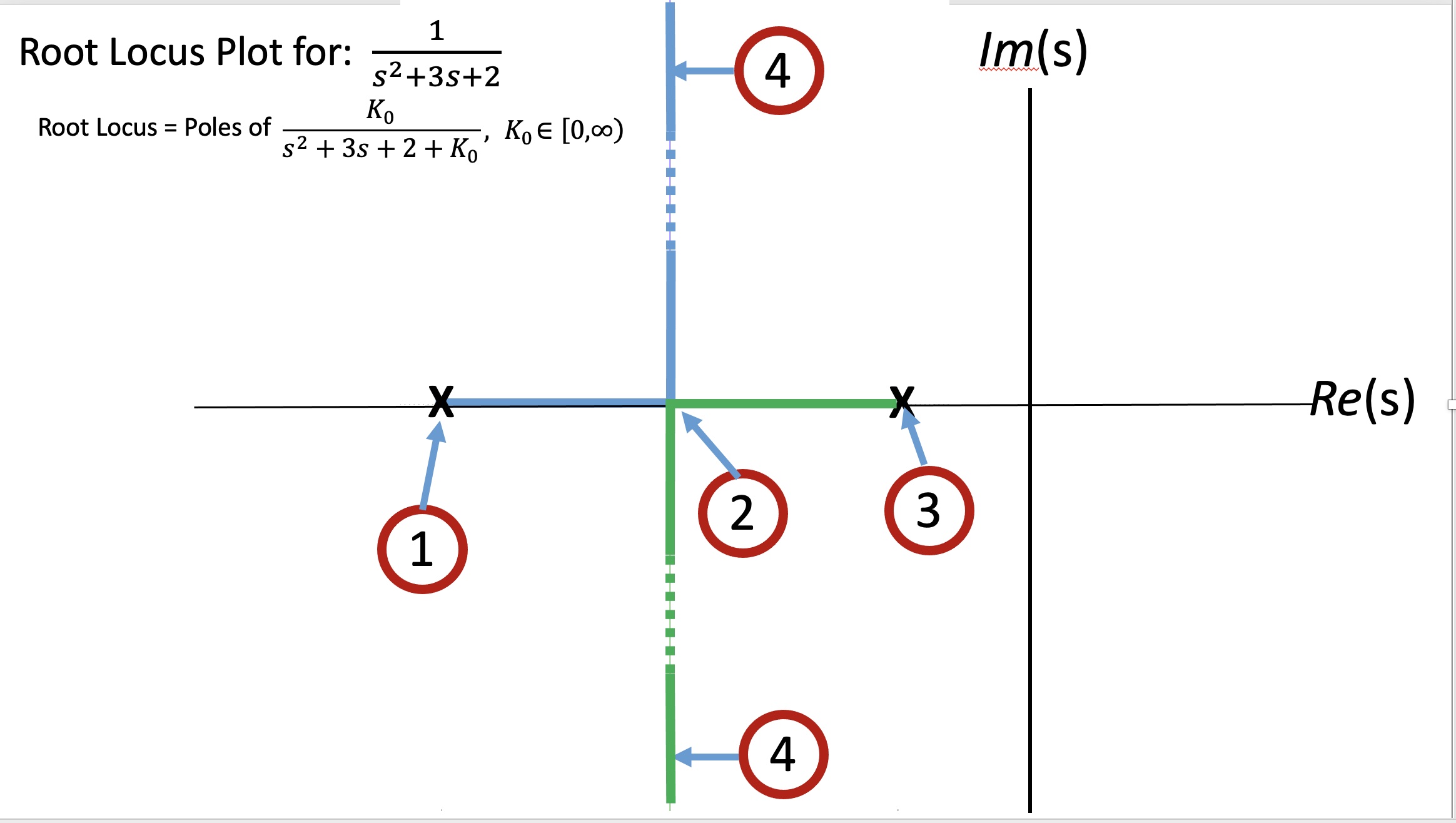
The figure above is a root locus plot for

K(s)H(s) = K_0 H(s) = \frac{K_0}{s^2 + 3s + 2}.

Where on the real line (denoted Re(s) in the above figure), are points 1, 2, and 3?

Re(s) for point 1

Re(s) for point 3

Re(s) for point 2

You will need to find G(s) to answer the following.

What K_0 Corresponds to point 2?

The root locus plot has a pair of points labeled 4 (a pair because real transfer functions have complex conjugate poles). What is the positive imaginary part of the poles at points 4? And what is K_0? For that you will need more information.

Consider the step response below, the imaginary part can be related to the period of oscillation, but hmmm, the time axis is missing. So the period is impossible to estimate, or is it? Can you use what you know about the the decay rate?

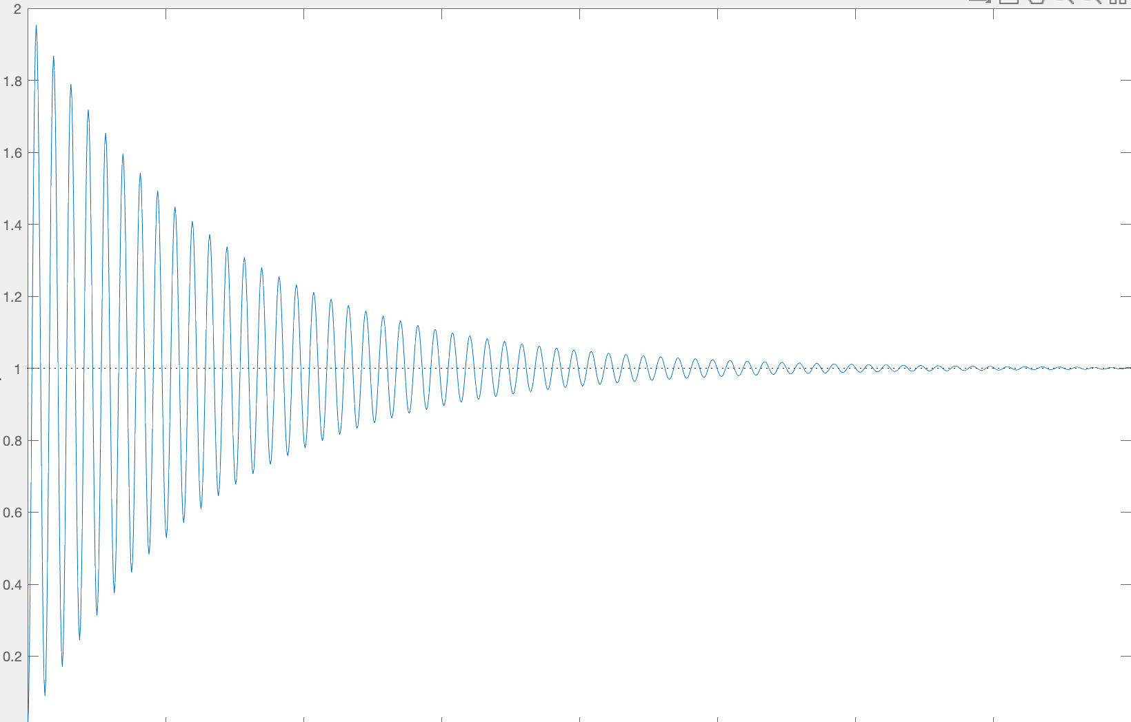
This is a relatively open-ended question. To answer it, think about what pieces of data you are given (i.e., the plot). What are you trying to extract? How will what you extract help you solve the problem?

What K_0 Corresponds to points 4 (to within 50 percent)?