Frequency-Response-Based Controller Design

1) A Long Prelab

This is a long prelab, intended to prepare you for the maglev design problem next week. It also introduces you to the matlab suite of computational tools for system analysis, tools which we will be using extensively for the remainder of the semester. We had intended to switch over to python exclusively this term, but that transition will have to wait until next term. We've had less time for development than expected, and we did not realize the diversity of python enviroments we would need to support. Our apologies for this, and we will try to make this change in plans as painless as possible.

You can use matlab on-line or install it on your computer, information on the alternatives for MIT students is available here. If you are new to matlab, we suggest using the on-line version, and there is a tutorial video here, but we will describe most of the commands you will need.

For this Friday's lab, if would help to skim over the matlab tools for creating CT transfer functions and computing step responses. But before beginning the design problem next week, you should finish this prelab.

2) Phase Margin and Leads

In much of the literature on linear systems analysis, the term "frequency domain analysis" is a very general catagory, and encompasses nearly every use of transforms to replace difference or differential equations involving functions of n or t, with rational functions (typically) of z or s. But when WE use the term "frequency response", we are referring to a system's eventual response to sinusoidal inputs as a function of the sinusoid frequency (the sinusoidal steady-state response). And we usually characterize the frequency response by its magnitude and angle (or phase) with respect to the input sinusoid.

When one uses frequency domain analysis to determine a stable system's transfer function, e.g. H(s), one generates a complex function of a complex variable s. The stable system's frequency response is given by H(s)|_{j \omega} = H(j \omega), a complex function of a real variable. And as a function of a real variable, frequency response can be characterized by easily-visualized plots of magnitude and phase versus \omega.

It is tempting to try to formalize these easily understood frequency response plots, and focus on connecting plot properties to guarantees about system performance. We will take an alternative approach, and instead focus on using frequency response as a tool for suggesting design alternatives. In particular, we will examine the notion of phase margin , show that good controllers have large phase margins, and show how to design candidate controllers that increase phase margin. But, while good controllers have large phase margins, having a large phase margin DOES NOT guarantee a good controller, so our candidate controllers must be verified.

Design is different from analysis, and is often more about generating worthwhile alternatives than providing a-priori guarantees. Assuming, of course, that one has the tools to verify any final design.

3) Matlab Tools for CT and Frequency Response.

You can use matlab to manipulate continuous-time transfer functions. First, you have to tell matlab to use s as the CT transform variable, by typing

>> s = tf('s')

After that, you can define a CT transfer function. For example, suppose your system is described by a set of differential equations

then assuming y(t) = Y e^{st} and x(t) = Xe^{st}, where H(s) is the CT transfer function given by

In matlab, if you type

>> H = (1/(s+0.1))*(1/s)*(1/s)

Matlab will response with

H =
 
        1
  -------------
  s^3 + 0.1 s^2

Then if you type

>> pole(H)

matlab will respond with poles (or natural frequencies),

ans =

         0
         0
   -0.1000

as you would expect since in CT, two of your poles are at zero.

We will make extensive use of the step, feedback, and bode commands. You can find information about any matlab command by typing, for example,

help step

to find out a little about the step command, or

doc step

to launch a documentation page with comprehensive information.

If you wanted a Bode plot of H(j \omega ) based on the H described above, you could type

bode(H)

As a more complete example, consider a system with input x(t) and output y(t) described by a first-order differential equation,

where y is the output and x is the input. Suppose we know that x(t) = \cos(\omega t) = \cos(2\pi f t) where \omega is the frequency in radians per second and f is the frequency in cycles per second. Approximately what is y(t) in the limit as t \rightarrow \infty ?

In this case, the system function is H(s) = \frac{1000}{s+1}. We say x(t) is equation to a unit step if x(t)=0 for t < 0, and x(t) = 1 for t \ge 0. To plot the response to the unit step using matlab, in the command window type (be sure you have defined s to matlab using s = tf('s')).

H = 1000/(s+1)

to define the system function to matlab, and then

step(H)

to plot y(t) given x(t) is a unit step. Note that y(t) rises to 1000 with a time constant of one second (about two-thirds of the rise in one second).

The frequency response of this first-order system can be plotted using

bode(H)

A Bode plot which labels the unity-gain (|H(j\omega)|=1) frequency, and its associated phase margin, can be plotted using

margin(H)

If we use feedback with this first order system, so that

then we can apply Black's formula to determine the closed-loop system function, G(s), If we set K(s) = 1, then We can also use matlab to determine the system function with the feedback command,

G = feedback(1000/(s+1),1)

In order to plot the locus of poles of G(s) as a function of K_0 of

you can use the root locus command

rlocus(1000/(s+1))

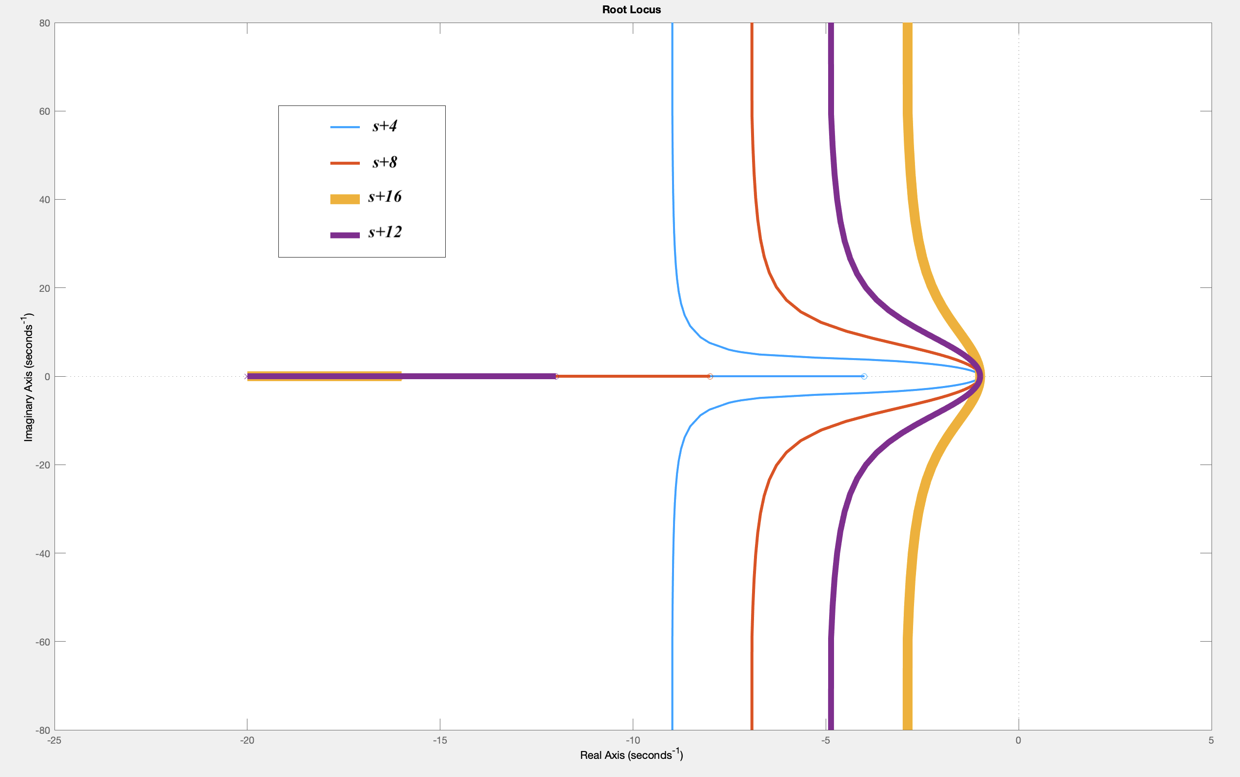
Root locus plots can be used to select a good controller. For example, for third-order system given by

we could use a controller with a single zero (or a proportional-derivative). To determine the best zero location, for example, we could use the following matlab commands to plot root loci for each of the controllers.

rlocus((s+4)/((s+20)*(s*s+2*s+1)))
hold on
rlocus((s+8)/((s+20)*(s*s+2*s+1)))
rlocus((s+12)/((s+20)*(s*s+2*s+1)))
rlocus((s+16)/((s+20)*(s*s+2*s+1)))

The above commands will generate a plot like the following (where we have recolored the lines and added a legend). Note that the controllers zeros at -4,-8,-12, and -16 generate root loci that have progressively less negative real parts, for worsening stability.

To plot the step response of the feedback system,

step(G)

The frequency response also shows the impact of including the first-order system in a closed loop, as can be seen in the plot generated by

bode(G)

For our third-order example, the step responses for the closed-loop systems can be compared, where notice that we have set a scale factor for each controller so that they all have the same steady-state value, K(j\omega)H(j\omega) for \omega = 0.

step(feedback((240*(s+4)/((s+20)*(s*s+2*s+1))),1))
hold on
step(feedback((120*(s+8)/((s+20)*(s*s+2*s+1))),1))
step(feedback((80*(s+12)/((s+20)*(s*s+2*s+1))),1))
step(feedback((60*(s+16)/((s+20)*(s*s+2*s+1))),1))

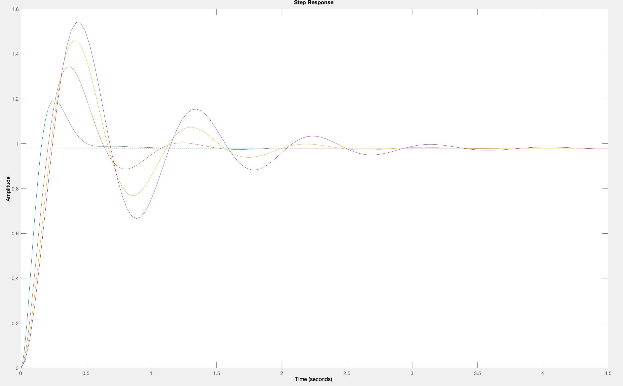
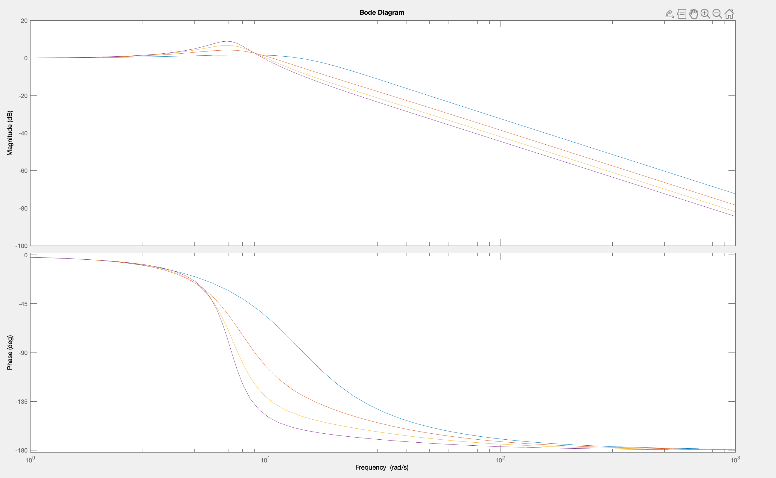
In the above plot, the step response for the s+4 controller has the smallest overshoot, unsurprising given the root locus plot. And what about the closed loop frequency response?

bode(feedback((240*(s+4)/((s+20)*(s*s+2*s+1))),1))
hold on
bode(feedback((120*(s+8)/((s+20)*(s*s+2*s+1))),1))
bode(feedback((80*(s+12)/((s+20)*(s*s+2*s+1))),1))
bode(feedback((60*(s+16)/((s+20)*(s*s+2*s+1))),1))

And the phase margin

margin(240*(s+4)/((s+20)*(s*s+2*s+1)))
hold on
margin(120*(s+8)/((s+20)*(s*s+2*s+1)))
margin(80*(s+12)/((s+20)*(s*s+2*s+1)))
margin(60*(s+16)/((s+20)*(s*s+2*s+1)))

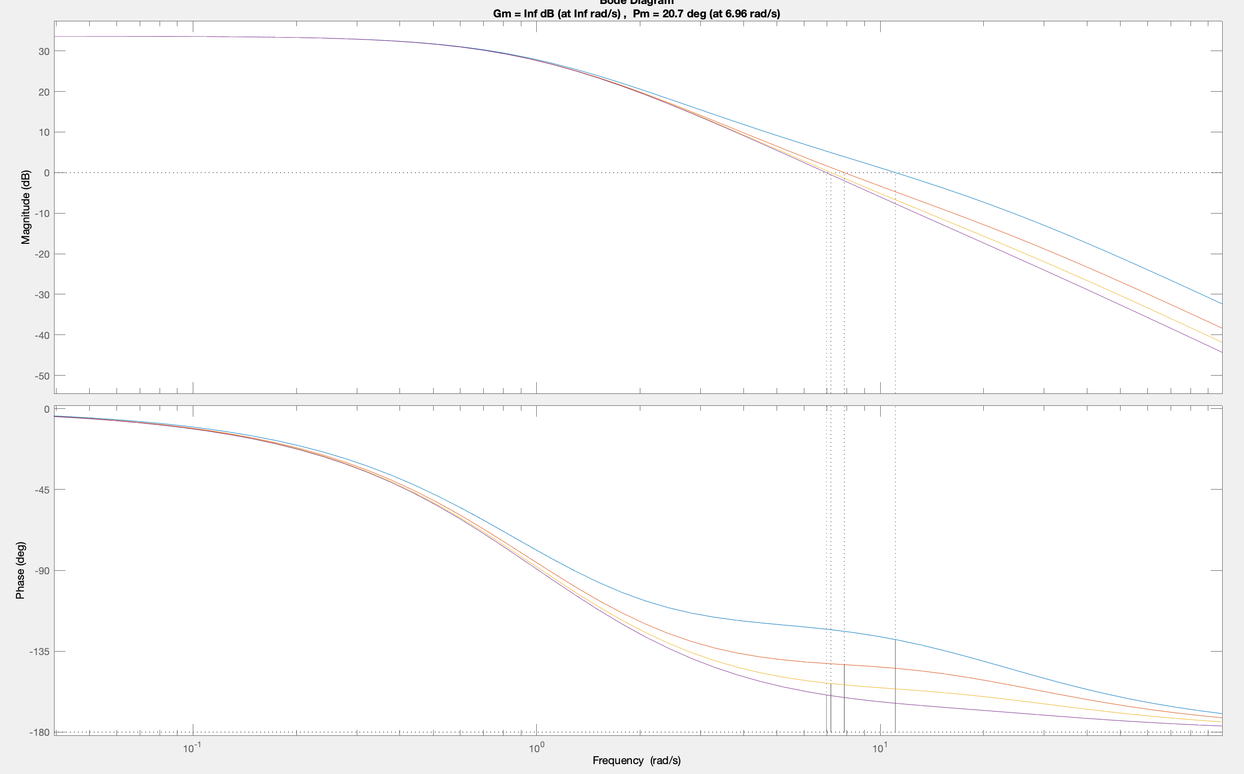
Notice that the s+16 controller resulted in a system whose step response had the most overshoot, whose frequency response had the most peaking, and whose phase margin was the smallest. Step response, closed-loop frequency response, and phase margin, they all they all tell the same story. The s+4 controller is more stable.

4) Example problems

• exercises: Lead Compensation (Due Apr 04, 2024; 10:30 PM)
• exercises: Bode and Steps (Due Apr 04, 2024; 10:30 PM)
• exercises: Arm Like Example (Due Apr 04, 2024; 10:30 PM)
• exercises: Phase Margin (Due Apr 04, 2024; 10:30 PM)