Eigenvalues to LQR

The questions below are due on Thursday April 25, 2024; 10:30:00 PM.

You are not logged in.
Please Log In for full access to the web site.
Note that this link will take you to an external site (https://shimmer.mit.edu) to authenticate, and then you will be redirected back to this page.

1) Revisiting the L-motor driven arm

Consider the L-motor driven arm described here , but this time, consider using LQR to design its controller.

2) The General LQR Setting

The input to any physical system we would like to control will have limitations that restrict performance. For example, we may be controlling a system by adjusting velocity, acceleration, torque, motor current, or temperature. In any practical setting, we will not be able to move too fast, or speed up too abruptly, or yank too hard, or drive too much current, or get too hot. And it may even be important to stay well below the absolute maximums most of the time, to reduce equipment wear. In general, we would like to be able to design our feedback control algorithm so that we can balance how "hard" we drive the inputs with how fast our system responds. As we have seen in the previous prelabs, determining k's by picking natural frequencies is not a very direct way to address that balance.

2.1) A Canonical Test Problem and a Sum-Of-Squares Performance Metric

Instead, consider determining gains by optimizing a metric, one that balances the input's magnitude and duration with the rate at which states of interest appoach a target value. And since our problems are linear, the metric can be established using a cannonical test problem, simplifying the formulation of the optimization problem. For the canonical test problem, we can follow the example of determining how the propeller-driven arm's position evolves just after being misaligned by a gust of wind. That is, we can consider starting with a non-zero initial state, \textbf{x}[0] , and then using feedback to drive the state to zero as quickly as possible, while adhering to input constraints. In particular, find \textbf{K} that minimizes a metric on the state, \textbf{x} , and the input, \textbf{u} = -\textbf{K} \cdot \textbf{x} , that satisify

\textbf{E} \frac{d}{dt}\textbf{x}(t) = \textbf{A}\textbf{x}(t) + \textbf{B}\textbf{u}(t) = (\textbf{A} - \textbf{B}\cdot \textbf{K})\textbf{x}(t).

And what is a good metric? One that captures what we care about, fast response while keeping the input within the physical constraints, AND is easily optimized with respect to feedback gains. The latter condition has driven much of the development of feedback design strategies, but the field is changing. Better tools for computational optimization is eroding the need for an easily optimized metric. Nevertheless, we will focus on the most widely used approach, based on minimizing an easily differentiated sum-of-squares metric.

The well-known linear-quadratic regulator (LQR) is a based on solving an optimization problem for a sum-of-squares metric on the canonical problem of driving \textbf{x}(t) to zero as quickly as possible given that x(0) \ne 0 . The optimization problem with metric for LQR is

\min_{\textbf{K}} \left( \int_{0}^{\infty} \textbf{x}^T(\tau)\textbf{Q}\textbf{x}(\tau) d\tau + \int_{0}^{\infty} \textbf{u}^T(\tau)\textbf{R}\textbf{u}(\tau) d\tau \right),

where \textbf{Q} and \textbf{R} are \#states \times \#states and \#inputs \times \#inputs positive definite state and input weighting matrices. The description of the optimization problem simplifies considerable if we consider the single input case with diagonal state weighting. If the system has n states, then diagonal state weighting means that the \textbf{Q} matrix is diagonal, as in

\textbf{Q} = \begin{bmatrix} Q_{1,1} & 0 & ... & ... & 0\\ 0 & Q_{2,2} & 0 & ... & 0 \\ ... & ... & ... & ... & ...\\ 0 & ... & ... & 0 & Q_{n,n} \end{bmatrix},

and the diagonal \textbf{Q} matrix is positive definite if Q_{i,i} > 0 for all i \in {1,...,n}. Given that there is only a single input, \textbf{u}(t) is a scalar, and the \textbf{R} matrix reduces to the scalar R_{1,1} > 0.

Rewriting the optimization problem for the single-input case with diagonal state weighting, we get

\min_{\textbf{K}} \left( \sum_{1}^{n} Q_{i,i} \int_{0}^{\infty} (x_i(\tau))^2 d\tau + R_{1,1} \int_{0}^{\infty} (u(\tau))^2 d\tau \right).

The first term

\int_{0}^{\infty} \textbf{x}^T(\tau) \textbf{Q}\textbf{x}(\tau) d\tau,

generally decreases when states go to zero faster, and the second term

\int_{0}^{\infty} \textbf{u}(\tau) \textbf{R}\textbf{u}(\tau) d\tau = \int_{0}^{\infty} \left(\textbf{K} \cdot \textbf{x}(\tau)\right)^T\textbf{R}\left(\textbf{K} \cdot \textbf{x}(\tau)\right) d\tau

generally increases when inputs have larger magnitudes and last longer.

By changing \textbf{Q} and \textbf{R} , one can trade off input "strength" with speed of state response, but only in the total energy sense implied by the sum of squares over the entire semi-infinite interval. In order to develop an intuition that helps us pick good values for \textbf{Q} and \textbf{R} , we will consider simplified settings.

The Matlab commands lqr and dss may be useful in working with LQR in state space, also think carefully about the value of the A, B, and C matrices when plotting multiple outputs in feedback.

3) LQR Weights, Gains, and State Trajectories.

Once we select a matrix of weights, \textbf{Q}, we can use matlab's lqr function to determine the associated feedback gains, but how do we select the weights? If we restrict ourselves to diagonal \textbf{Q}'s (only the Q_{i,i}'s are non-zero), then it is a little easier to develop some intuition.

Consider our example three-state, single-input, motor-driven arm system. If we use lqr with diagonal weights to determine its feedback gains, the gains will solve the optimization problem,

\min_{\textbf{K}} \left( \int_{0}^{\infty} \sum_{1}^{3} \textbf{Q}_{i,i} (x_i(\tau))^2 d\tau + \int_{0}^{\infty} R_{1,1} (u(\tau))^2 d\tau \right),

where \textbf{x} satisfies the motor-arm differential equation system with nonzero initial state, \textbf{x}(0), and with u = - \textbf{K} \textbf{x}, (so y_d = 0). You might be surprised to learn that the minmizing \textbf{K} usually does not depend on the specifics of the non-zero initial state, a topic we defer to your next control class.

3.1) Minimization and Step Responses

Since the cost function in the above minimization can be infinite if the closed-loop system is unstable, the above minimization will find a stabilizing \textbf{K} if one exists. But otherwise, the above decay-to-zero senario seems inconsistent with the most common way we assess feedback controller performance, by examining step responses.

When computing a step response for our closed-loop system, we start from the zero initial state, and if the system is stable, watch as the state transitions to a nonzero steady-state in response to a given step change in y_d. We will denote this non-zero step-response steady-state as

\lim_{t \rightarrow \infty} \;\;\ \textbf{x}(t) = \textbf{x}_{ss}.

Since we often want to find feedback gains that accelerate the approach to the step response's steady-state, why pick gains that minimize decay from an initial state? Specificially, in our three-state system, it might seem more natural to find gains that solve the optimization problem

\min_{\textbf{K}} \left( \textbf{Q}_{1,1} \int_{0}^{\infty} (x_1(\tau)-x_{{ss}_1})^2 d\tau + \textbf{Q}_{2,2} \int_{0}^{\infty} (x_2(\tau) - x_{{ss}_2})^2 d\tau + \textbf{Q}_{3,3} \int_{0}^{\infty} (x_3(\tau) - x_{{ss}_3})^2 d\tau + R_{1,1} \int_{0}^{\infty} (u(\tau) -u_{ss}) d\tau \right),

where \textbf{x}_{ss} is the nonzero step-response steady-state, and u_{ss} = -\textbf{K}\textbf{x}_{ss}.

With a little careful though, it is easy to see that for a linear state-space system, the above two formulations have exactly the same minimum with respect to \textbf{K}. But when trying to determine good values for the \textbf{Q} weights, it is often easier to think in terms of minimizing the time spent away from steady state.

Suppose we use LQR to design a controller for the motor-driven arm. We might put a large Q weight on the arm angle state, so that the gains produced by LQR will result in a closed-loop system in which the arm moves rapidly to its steady-state. And since the rotational velocity state is zero both at steady-state and initially, if we put a large Q weight on the rotational velocity state, the gains produced by LQR will result in a closed-loop system in which rotational velocity is always kept small, and the arm will move slowly. Note, a high weight on both the angle and the velocity states counter-act each other to some degree, but not entirely. A high weight on the angle state will ensure that the actual arm angle will be an accurate match to the desired angle, at least in steady-state.

Can one can develop a similar intuition for the effect of increasing the Q weight on the motor current state? Partly yes, because of the relation between motor current and arm rotational acceleration. A high Q weight on the arm acceleration state will lead to a control system which can only deccelerate slowly, leading to significant overshoot. But, the step-response steady-state for motor current is not necesssarily zero (e.g. if there is a rubber band on the motor arm), and this makes determining the impact of high weight on motor current more complicated than determining the impact of high Q weight on rotational velocity.

3.2) Guess the Weights.

In this problem, we practice using the above intuition by determining the impact on state trajectories of using various Q-weights when designing an LQR-based controller for the Lmotor-driven arm. As above, we will restrict overselves to considering only the diagonal "Q"-weights, \textbf{Q}_{1,1}, \textbf{Q}_{2,2}, and \textbf{Q}_{3,3}. Also, since we are investigating how the relative state weights affect the resulting gains and therefore, closed-loop behavior, we will normalize the input weight, and set R_{1,1} = 1.

In order to generate a set of interesting cases, we assigned each of three weight values, 1, 10 and 100, to one of the three "Q"-weights, \textbf{Q}_{1,1}, \textbf{Q}_{2,2}, and \textbf{Q}_{3,3}, and used lqr with those Q weights (and an R weight of one) to determine the state-feedback gains (and the associated K_r). Below are plots of the three state trajectories in response to a unit step input for each of the six weight distributions. Your job will be to figure out which trajectory goes with which system. But remember, you are looking at step responses which have non-zero steady states. That may be obvious when considering the arm angle, but as the plot labeled Case C clearly indicates, the motor current also has a non-zero steady state.

We encourage you to try to reason out the solution to this problem, but matching behavior to the correct weight combination can be tricky. Do the best you can, but if you can not get the right answer in a few tries, you can resort to matlab for some help. You can use matlab's lqr command to determine the gains, then create a closed loop system using matlab dss command, and finally use matlab's step command to plot step responses of the generated system (though you will need to create a special \textbf{C} matrix with multiple rows to force the step function to plot all the states). You can also compute the step responses of all the states in a system with the following Matlab snippet. (Do you see the reason for the identity matrix Cstate?)

s = tf('s')
figure(1)
step(C*(inv(s*eye(3)-A)*B))
Cstate = eye(3)
figure(2)
step(Cstate*(inv(s*eye(3)-A)*B))

Below are the plots of controller step responses for the matching.

Case A

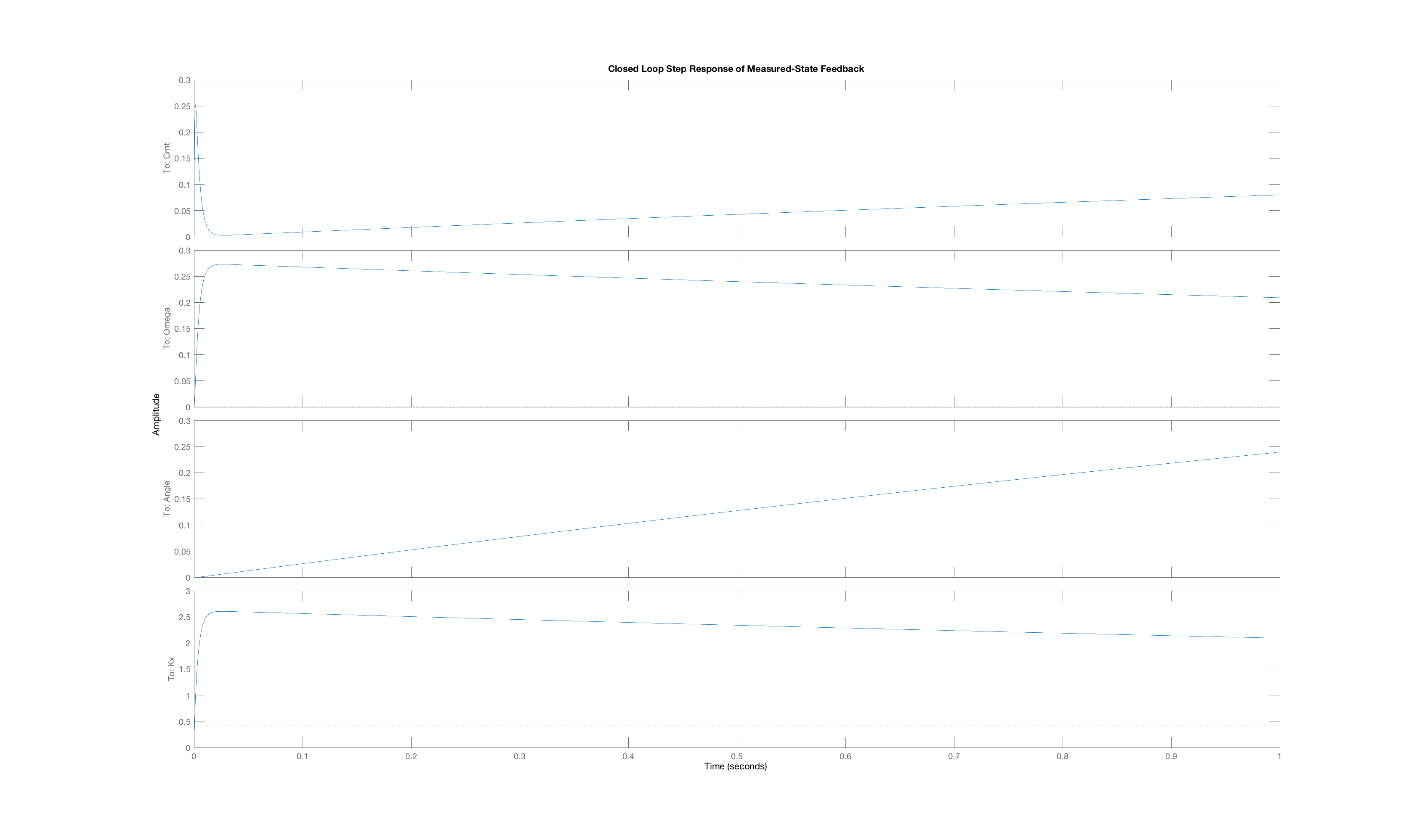
Case B

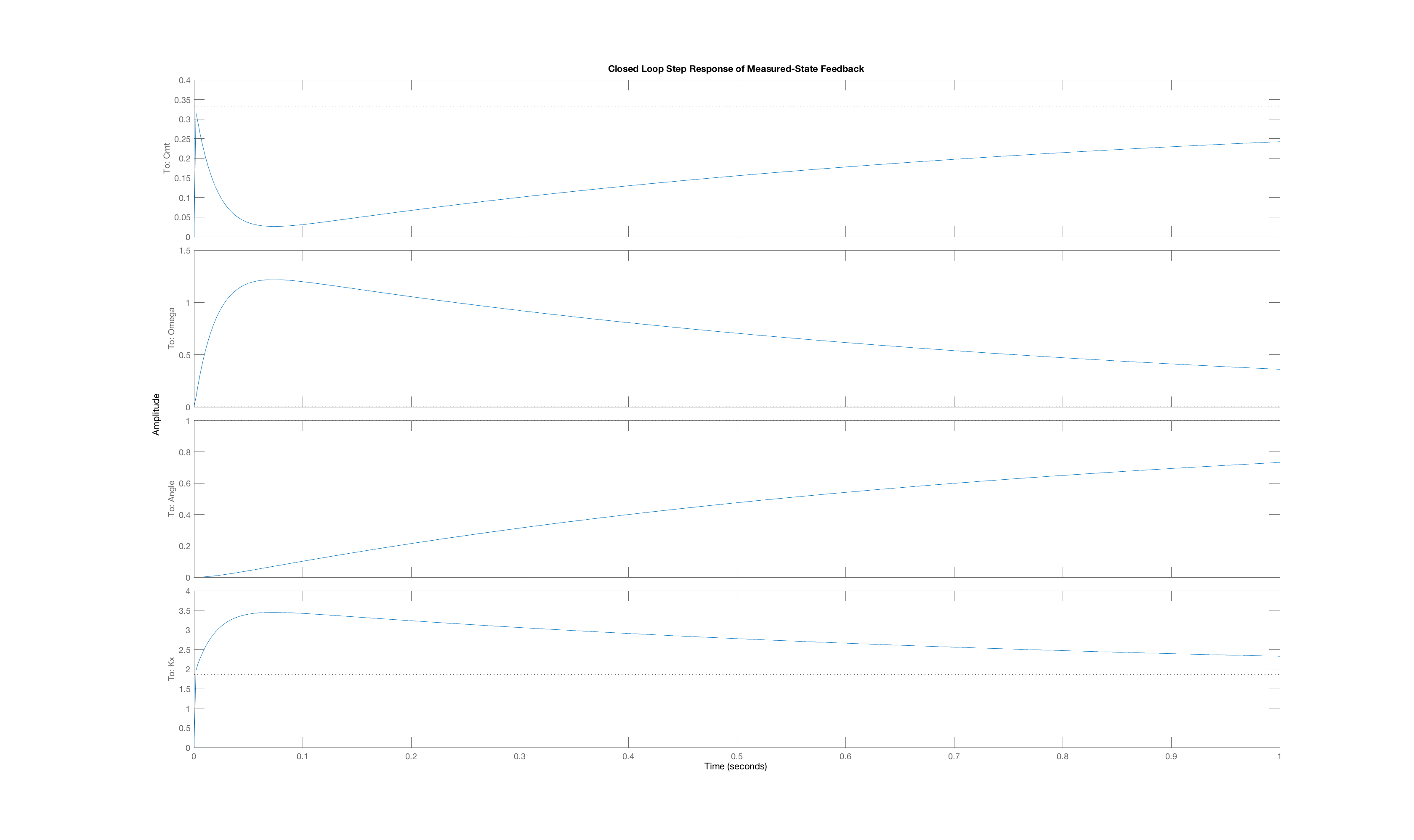
Case C

Case D

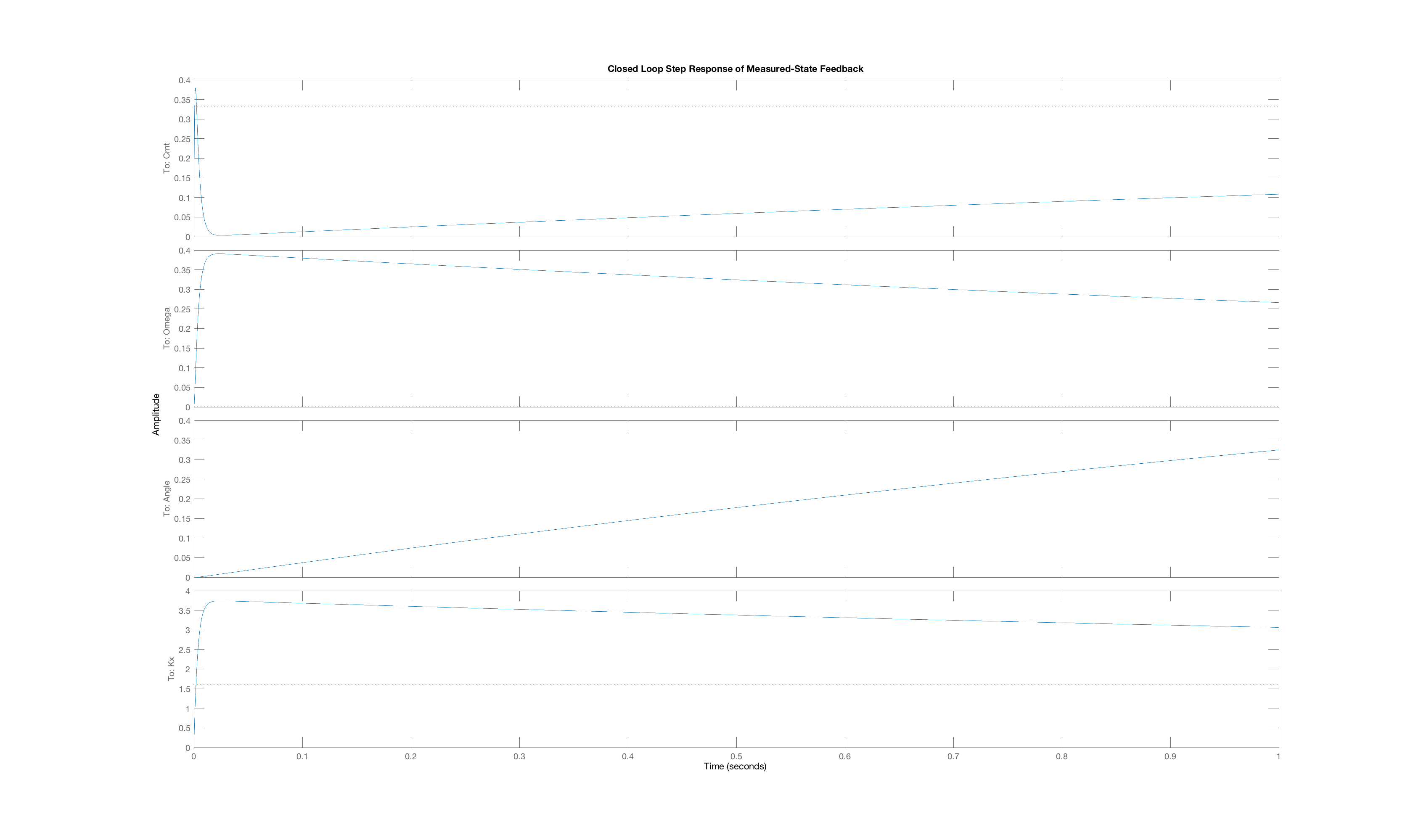
Case E

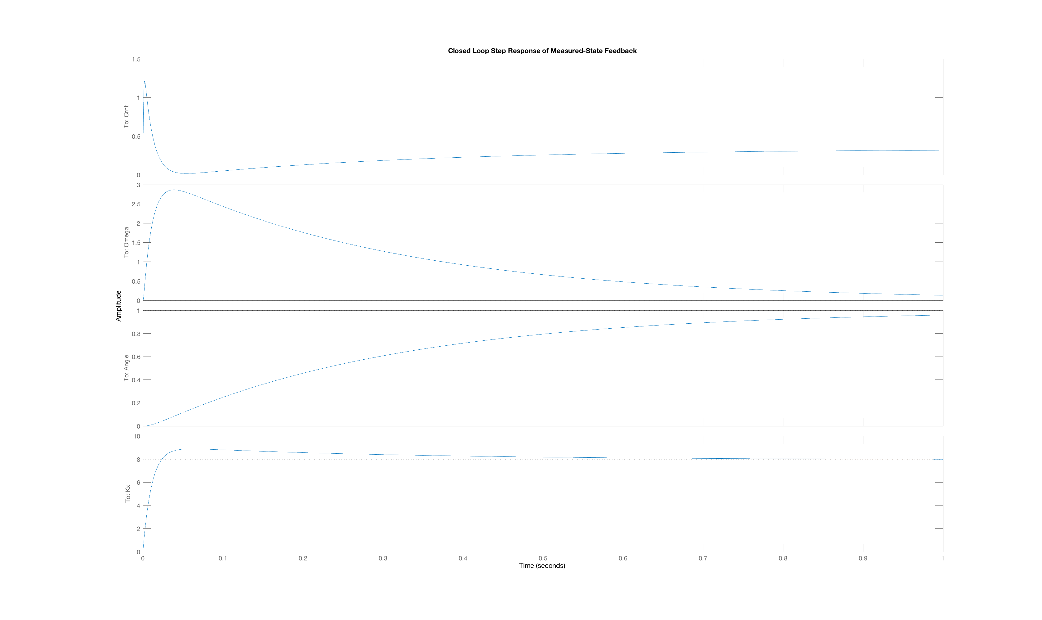
Case F

The six plots A to F above correspond to six sets of Q weights,

[\textbf{Q}_{1,1}, \textbf{Q}_{2,2}, \textbf{Q}_{3,3}] = [1,10,100], [10,1,100], [1,100,10], [100,1,10], [10,100,1], [100,10,1].

Order the plots using their letters so that the plot order matches the "Q"-weight order in the above list. That is, if you fill in the answer

ABCDEF

then you mean that plot A is the closed-loop step response for LQR gains picked with diagonal weights [1,10,100], and B goes with [10,1,100], etc.

Plot Order =

Once you have defined the \textbf{E}, \textbf{A}, and \textbf{B}, matrices for the Lmotor-driven arm in matlab, you can use the matlab lqr command to compute the vector of state feedback gains given the "Q"-weights on the three states,

[\textbf{Q}_{1,1}, \textbf{Q}_{2,2}, \textbf{Q}_{3,3}] = [5,25,125],

and "R"-weight on the scaler input,

\textbf{R}_{1,1} = 1.0,

using the matlab command

K = lqr(E\A, E\B, diag([5,25,125]), diag([1.0])

Suppose we use LQR to compute the gains for a state-feedback controller for the Lmotor-driven arm, with and without rubber bands. If the state-feedback gains are computed with an "R"-weight of 1.0 and one of the six sets of diagonal "Q"-weights

[\textbf{Q}_{1,1}, \textbf{Q}_{2,2}, \textbf{Q}_{3,3}] = [1,10,100], [10,1,100], [1,100,10], [100,1,10], [10,100,1], [100,10,1],

(note that these are the weight sets from the problem above) then what can you say about the poles for the twelve closed-loop transfer functions?

If you have defined \textbf{E}, \textbf{A} and \textbf{B} for the with-rubber-bands case and the no-rubber-bands case, you can use the following snippet of matlab code to display the poles for six closed-loop controllers

Qv = [1,10,100;1,100,10;10,1,100;10,100,1;100,1,10; 100,10,1];
for i = 1:6
   K = lqr(E\A,E\B,diag(Qv(i,:)),1.0);
   display(eig(E\(A-B*K)).');
end

Twelve closed-loop transfer functions were generated using the six sets of "Q"-weights and the with- and without-rubber-bands. The poles of all the closed-loop systems generated using the LQR-computed gains are all negative and real. Why is that?

	The poles of closed-loop systems generated using LQR-computed gains are always real and negative
	If an open-loop system has negative real poles, then the poles of the closed-loop system generated using LQR-computed gains are always real and negative
	The metric being minimized by LQR is lower if the states in the closed-loop system decay more rapidly, and that favors poles with more negative real parts, but there are no guarantees

Suppose we change all the weights by scaling by an integer k, as in

Qv = k*[1,10,100;1,100,10;10,1,100;10,100,1;100,1,10; 100,10,1];'

If we scale all the weights, what is the minimum value of k for which at least one of the twelve systems has at least one pole with a non-zero imaginary part.

Minimum integer weight scaling:

Scaling all the weights together can accelerate the system, but to really change the character of the system, we need to change the relative weighting of the states. So, suppose we replace only the weights of 100 by weights of k*100, as in

alpha = k*100;
Qv = [1,10,alpha;1,alpha,10;10,1,alpha;10,alpha,1;alpha,1,10; alpha,10,1];

By scaling only one state weight, we can more easily change the character of the system. For this one-scaled case, what is the minimum value of k for which at least one of the twelve systems has at least one pole with a non-zero imaginary part.

Minimum integer weight scaling:

When a stable system has complex poles, those poles have negative real parts, so the associated time-domain behavior is a decaying oscillation,

e^{-real(\lambda)t}cos(imag(\lambda) t + \phi).

where \lambda is the complex pole. For the oscillations to be visible, the oscillation period has to be small compared to the time constant associated with the decay, so imag(\lambda) must be significantly larger in magnitude than real(\lambda). For the two scaling cases above, the feedback systems we generated did have poles with imaginary parts, but those imaginary parts were much smaller than the real part, so no oscillations were visible.

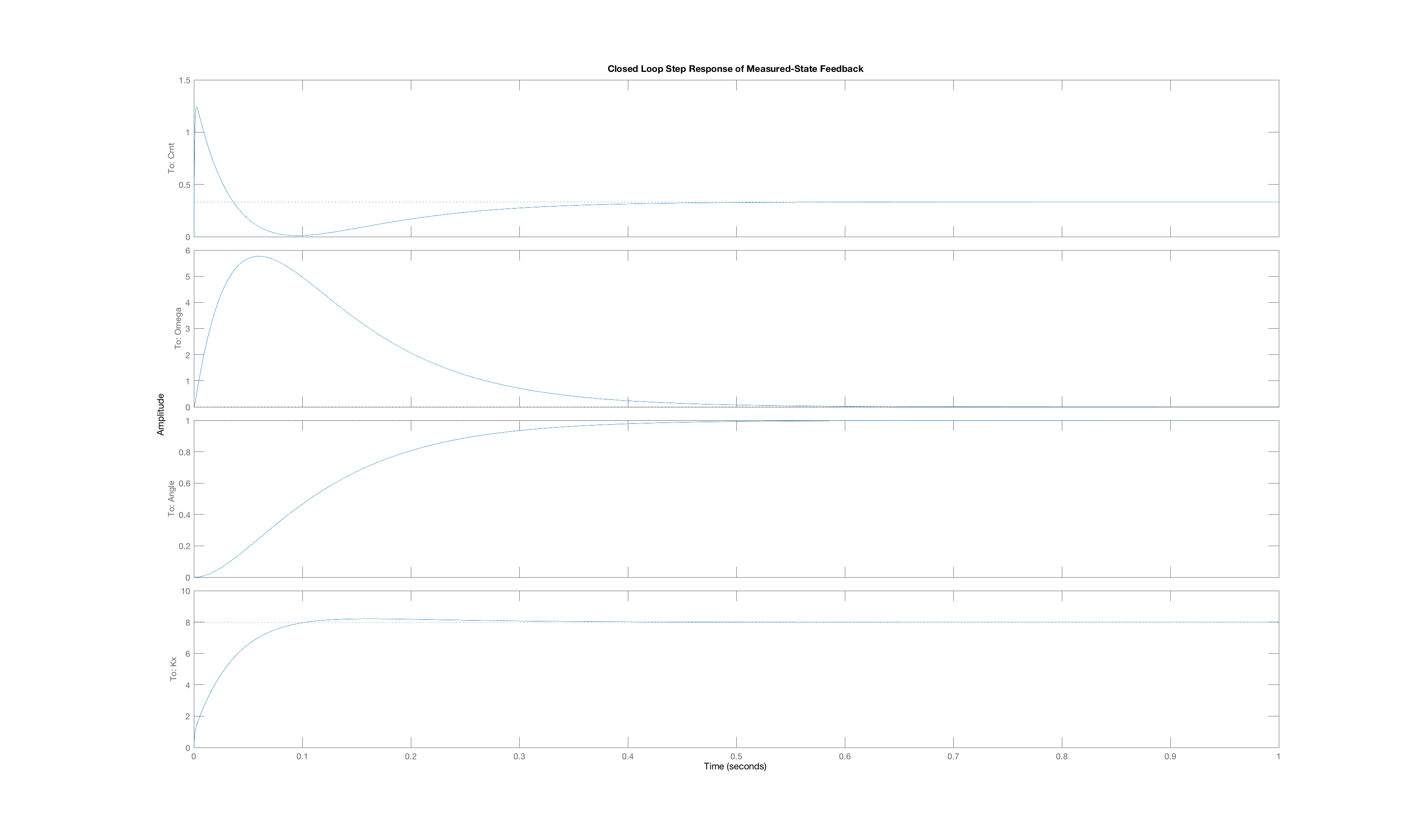
One has to pick ridiculous weights to convince LQR to produces gains that lead to state-feedback systems with highly imaginary poles, but for the Lmotor-driven arm with rubber bands, we did succeed. We used diagonal state weighting, and set two of the weights to 1.0, and the third to 10^p, where p is an integer larger than 2 (you will have figure out what p is, and which state was given a high weight). We then generated a feedback system using the generated gains, and examined the poles. One pole was real and very fast, with a value of -20,000, and the other two poles formed a complex pair, at -1.1 +/- 8.1j. The behavior of this intentionally poorly-designed feedback system is shown below, where the oscillations are very clear.

What LQR weights produced the gains used in our oscillatory

Which state was given a high LQR weight?

	motor current
	Omega
	Theta

We set the one large weights to 10^p for some integer p, what is p?