Pendulum Two-State Example

The questions below are due on Thursday April 25, 2024; 10:30:00 PM.

You are not logged in.
Please Log In for full access to the web site.
Note that this link will take you to an external site (https://shimmer.mit.edu) to authenticate, and then you will be redirected back to this page.

1) Pendulum

Imagine a pendulum suspended from tree trunk, swaying thanks to occasional torque forces generated by gusts of wind. We can generate a state-space model for the pendulum by treating it as a point mass, accelerated by a vector sum of forces, as in the figure above.

Denoting \theta as the angle of the pendulum, then \omega=\frac{d}{dt}\theta is the pendulum's angular velocity and \alpha = \frac{d}{dt}\omega is the angular acceleration. We use J to denote the moment of inertia (which, in the case of our point mass, is ml^2), T to denote the applied torque, l to denote the distance between the pivot and the point mass, and m to denote the mass of the point.

Newton's Second Law applied to the pendulum yields,

T - mgl\sin\theta = \alpha J.

Linearizing about the pendulum's nadir, \theta = 0, we have

T - mgl\theta = \alpha J,

as \frac{d}{d\theta} \sin\theta = \cos\theta = 1 at \theta = 0.

The moment of inertia is related to the point mass, J = ml^2, and angular acceleration is the derivative of angular velocity, \alpha = \frac{d}{dt}\omega. Substituting those relations,

\frac{d}{dt}\omega = -\frac{g}{l}\theta + \frac{T}{J}.

We can assemble the differential equations above to generate the \textbf{A}, \textbf{B}, and \textbf{E} matrices for the standard state-space descriptor form

\textbf{E}\frac{d}{dt}\textbf{x} = \textbf{A}\textbf{x} + \textbf{B}u

as in

\begin{bmatrix}1 & 0\\0 & 1\end{bmatrix} \frac{d}{dt} \begin{bmatrix}\theta \\ \omega\end{bmatrix} = \begin{bmatrix}0 & 1\\-\frac{g}{l} & 0\end{bmatrix}\begin{bmatrix}\theta \\ \omega\end{bmatrix} + \begin{bmatrix}0 \\ \frac{1}{J} \end{bmatrix}T

where E and A are 2x2 matrices, B is a 2x1 matrix, and more specifically, E is the two-by-two identity matrix.

For a complete state-space description, we also need an output equation involving \textbf{C} and \textbf{D} matrices, as in

y = \textbf{C}\textbf{x} + \textbf{D}u.

but in almost all of our examples, \textbf{D} = 0, because quantities like force are rarely algebraically related to quantities like position.

2) Output Matrices

If we wish the single output of our system to be pendulum's angle, what would the \textbf{C} and \textbf{D} matrices be? Enter the \textbf{C}, \textbf{D} matrices below for the state space representation above, assuming that the input to the system, u, is the applied torque, T, and the observed output, y, is equal to the angle \theta. (Remember to use Python form. If \textbf{C} is \begin{bmatrix}1 & 15\end{bmatrix}, you should enter [[1,15]], and be careful to give the correct brackets for \textbf{D}, even though its numerical values are all zero.

3) Damping

Friction force due to air resistance, usually modelled as being linearly proportional to rotational velocity, will dampen the oscillations of the pendulum. Friction damping is an extra force and is added to the linearized newton's second law equation,

T - mgl\theta - \beta \omega = J\alpha,

where \beta is the friction coefficient and \beta \omega is the friction force. Substituting for acceleration and moment of inertia,

\frac{d}{dt}\omega = \frac{T}{J} - \frac{g}{l}\theta -\frac{\beta \omega}{J}

since \omega = \frac{d}{dt}\theta, \alpha=\frac{d}{dt}\omega, and J = ml^2.

Note that by including friction, the angular acceleration includes a direct dependence on angular velocity, so the lower right corner of the \textbf{A} matrix is non-zero.

If we were to add damping to the system, what matrix would that modify?

	A
	B
	C
	D
	E

4) Poles with and without Damping

As discussed in lecture, when analyzing our state space model in the s domain, the poles of the system are the eigenvalues of the system matrix \textbf{A} (assuming \textbf{E} is the identity matrix). Those eigenvalues can be determined computing the values of s for which the determinant of \left(s\textbf{I} - \textbf{A}\right) is zero. That is, the poles are all values of s for which

\det\left(s\textbf{I} - \textbf{A}\right)=0.

If the \textbf{E} matrix is not the identity, then the system is a true descriptor system (with a \begin{bmatrix}E\end{bmatrix}), and the poles are equal to the generalized eigenvalues. That is, the poles of the system are all values of s such that

\det\left(s\textbf{E} - \textbf{A}\right)=0.

The techniques used to computing eigenvalues for large matrices never (almost never) involve using determinants, but for 2 \times 2 matrices, finding eigenvalues by computing determinants helps develop intuition and insight.

Suppose you are given the following system parameters, use them to answer the questions below.

m = 1\text{ kg}
l = 1\text{ m}
g = 9.81\text{ m}\cdot \text{s}^2
\beta = 0.02\text{ kg}\cdot \text{s}^{-1}

What are the two poles for the undamped(original) system?

What are the two poles for the damped system?

5) Using State Feedback to Stabilize the Pendulum

If we put the system we have into feedback like that shown below:

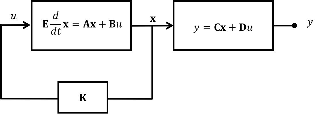
We actually gain the ability to move the poles around because where before we assumed the input to the system was nothing (u=0), we're now saying that the input is based off of the state multiplied by some gain vector \textbf{K}. This means our new expression for the system poles is:

\det\left(s\textbf{E} - \left(\textbf{A}-\textbf{B}\textbf{K}\right)\right)=0

For the undamped system, determine a set of gains K_1 and K_2 where \textbf{K} = \begin{bmatrix}K_1 ~~ K_2\end{bmatrix} to move the poles of the system in feedback so that they are both equal to -4.

K_1=

K_2=