Code Of Arms
Please Log In for full access to the web site.
Note that this link will take you to an external site (https://shimmer.mit.edu) to authenticate, and then you will be redirected back to this page.
Quick Reference
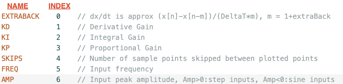
Serial Plotter Send Window Indices
Links
- Build instructions are here.
- Sketch for this lab is here.
- Matlab script for week B, rootPlotLab02.m
Task Summary
- Build, Calibrate, and Test the Arm Control System (Checkoff 1).
- Investigate the behavior of your arm when using only proportional feedback, K_p, and examine the behavior of difference estimates of the derivative as you change the difference interval m (Checkoff 2).
- Relate difference equation natural frequencies to measured arm behavior, and use the relation to estimate \gamma_a in a 2nd-order model of the arm (Checkoff 3).
- Investigate, experimentally, relationships between proportional and derivative feedback gains and arm performance. Pay particular attention to determining when step responses show the impact of nonlinearity.
- Learn to use a matlab script for computing poles and step responses, and use it to determine a range of gains for which the natural frequencies of your previously calibrated 2nd-order model is consistent with measured behavior (Checkoff 4).
- Extract \gamma_a and \beta_a coefficients from small-amplitude step response data for a PD controller with a non-instant 1st-order difference equation model of the command-to-thrust relation. Examine results from using large stepsizes.
- Add integral feedback to your model, and use the model to design a good PID controller. Compare with experiments, and then investigate how the integral term effect steady-state errors when you introduce disturbances (checkoff 6). Take screen shots with and without the integral term for the POSTLAB!
Introduction
In the last lab you modeled and determined control parameters for a motor speed control system, a relatively stationary example, and in this lab you will fly! Well, maybe "fly" is a bit of an exaggeration, though there will be motion. You will build a propeller-thrust-driven rotating arm, and you will control the arm's position by using angle measurements to adjust propeller motor drive. Perhaps a few videos...
Arm Wrestling
In the videos above, we show three propeller arm control systems. In the top video, we show what would happen if we used the same proportional feedback controller we used for speed control. In the bottom left, we show a video of using a PID controller, like the one you will be able to design by the end of this lab. And in the bottom right picture, we show you the kind of controller you will be able to design by the end of the term (after we cover state-space and observers).
The Key Challenge
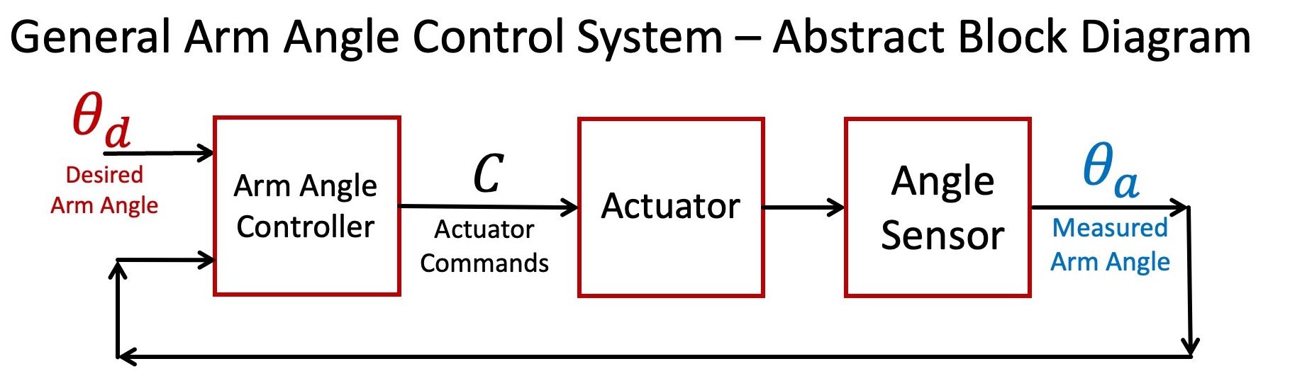
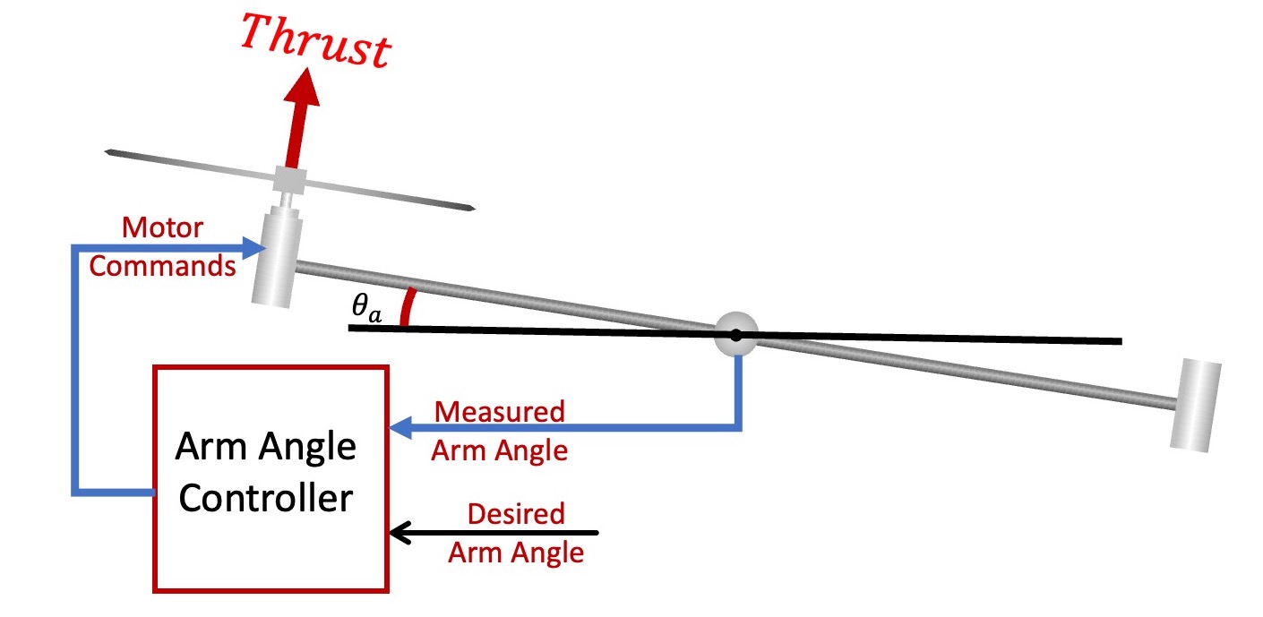
As the abstract block diagram (left panel above) suggests, controlling the rotation angle requires three interconnected functions, an actuator, a sensor and a controller. The angle sensor generates an analog voltage proportional to rotation angle, which is much more direct than the optical encoder sensor used for speed control. But the actuator is more complicated (right panel above). The controller sends commands to the motor and the resulting motor speed generates thrust on the rotating arm. The thrust accelerates the arm. The acceleration induces a change in arm velocity. And the arm velocity changes the arm angle. The layers of indirection make the control problem challenging, but not uncommonly so, most systems using force-based actuators are similar.
Control Design Approach
Like before, you will model your system and then use the model to help determine a good controller, though for the arm angle control, the modeling and controlling is more complicated. So, you will start with a simple proportional feedback controller, measure the arm behavior, and use those measurements to calibrate a second-order difference equation model of the arm. Then you will use your arm model to determine how the controlled-system's natural frequencies change as a function of proportional(P) and delta(D) (or derivative) feedback gains, and use that insight to design a good PD controller. Success! -ish.
It is possible to find an "okay" PD controller using the second-order arm model, a model accurate enough to predict failure for proportional-only control, but not much more. To achieve better performance, you'll need a more sophisticated controller, and to tune it, you will need a more comprehensive arm model. In particular, you will add an integral (or summation) term to your controller (the "I" in PID), and then tune the three gains (proportional, K_p, derivative, K_d, and integral, K_i) using a model that includes a non-instant relation between changes in motor command and the resulting changes in propeller thrust. And to analyze this complicated controller and model system? For that, you will need to make use of the more sophisticated analysis techniques you've just learned.
Assemble and Test
Please build the propeller-arm control system as described here. Be sure to complete the testing at the end of the assembly guide so that:
- the angle sensor axle is oriented correctly,
- the measured angle displayed by the serial plotter is zero when the arm is horizontal,
- and you've adjusted the nominal motor command so that the associated propeller thrust holds the arm level (that is, horizontal).
Demonstrate your calibrated arm.

Experiment with Proportional Gain
For the second checkoff, we would like you to try some preliminary experiments with proportional feedback, to help you develop an appreciation for the differences between the arm angle and speed control problems.
Determine how the response of the system changes with K_p by using the following procedure:
- Use the send window to set K_p (type "3 0.6" for example).
- Hold the arm (with your hand) so that the serial plotter shows the arm is about 60 milliradians above horizontal.
- Be prepared to stop the plotter -- then let go of the arm!
- Stop the plotter, then stop the arm by grabbing the end of the chop stick or by pulling the large power connector.
- Repeat with a new K_p
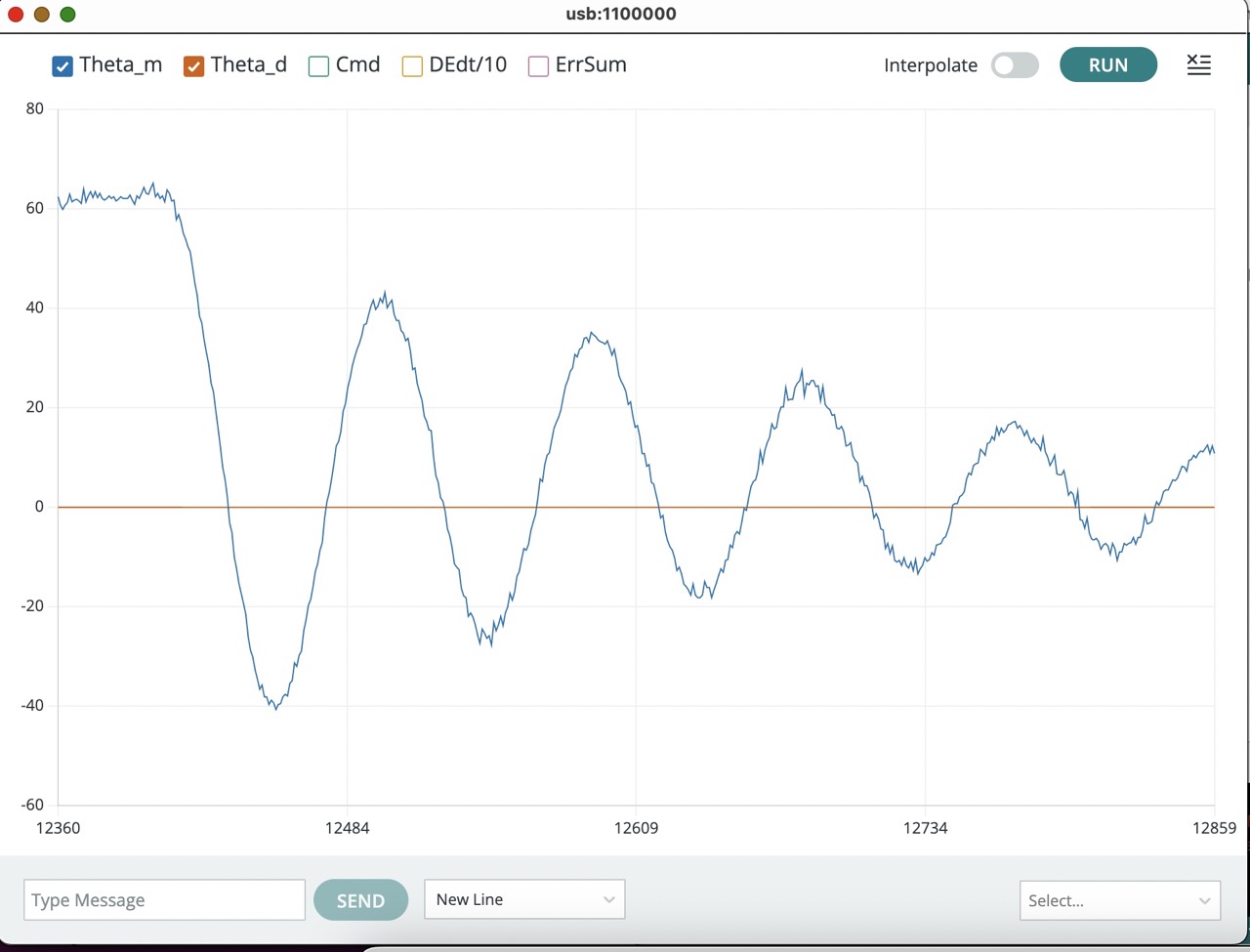
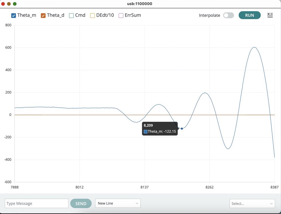
You should be able to find K_p's in the range \frac{1}{4} < K_p < 2 that produce both stable and unstable oscillating behaviors (like the two figures below). Try to find one that is stable (decays to zero like the first figure below), and one that is unstable (like the second figure below). Take screen shots for these two behaviors. You will need them for the checkoff.
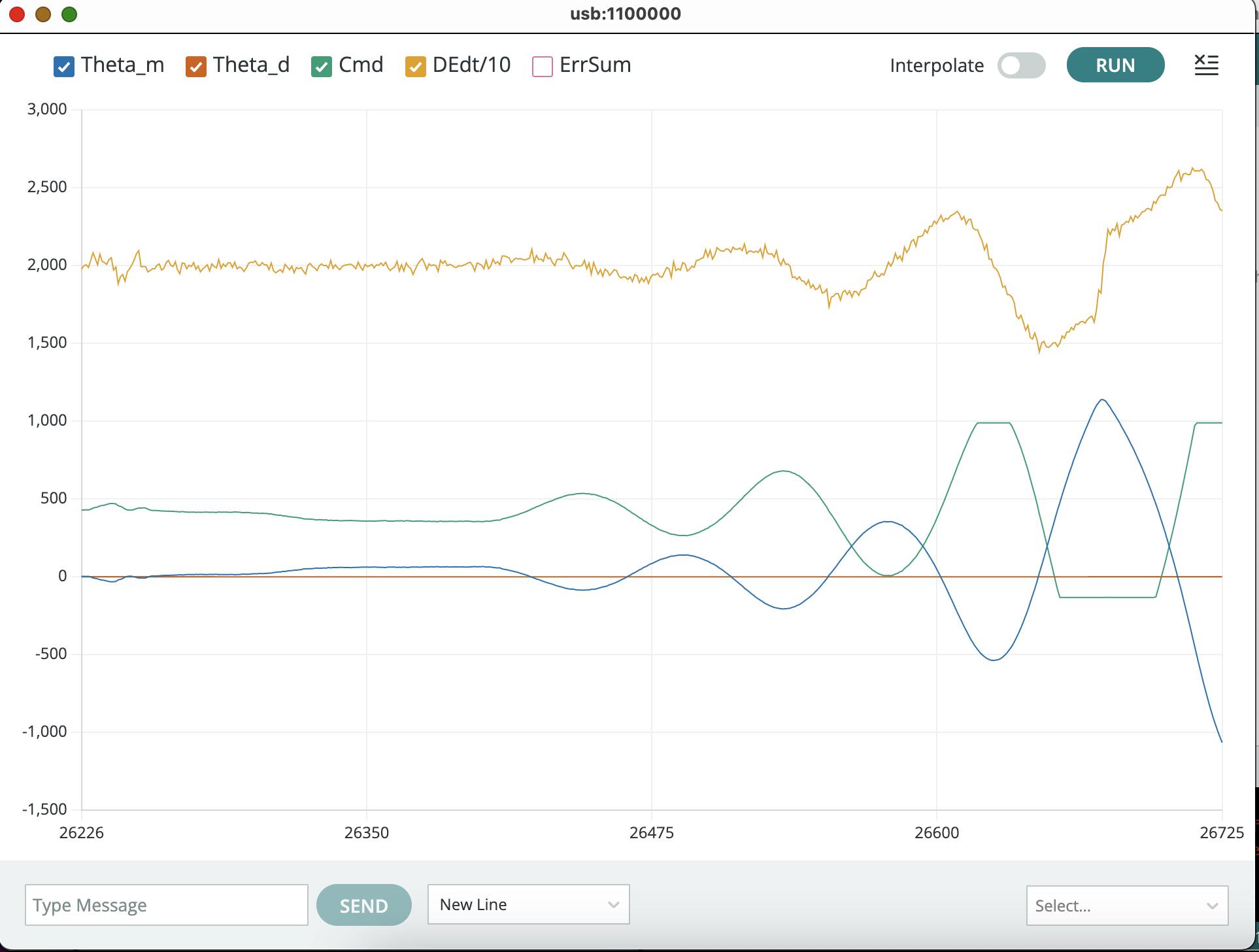
Examining Cmd and DEdt/10
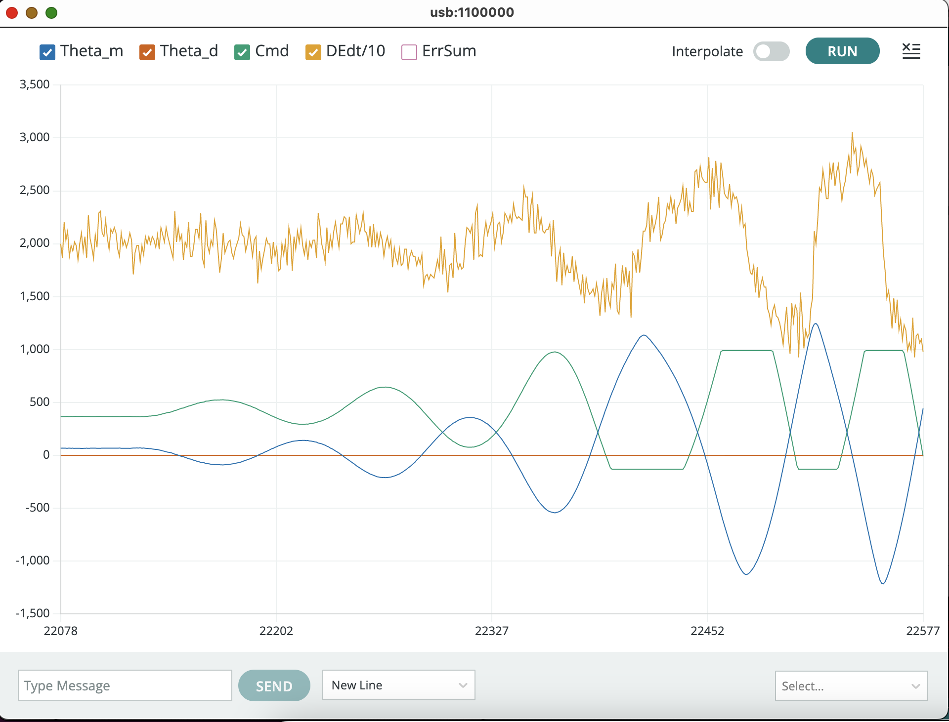
Once you have found a pair of K_p's (one producing decaying, and the other growing, oscillations), turn on the serial plotter plots for the motor command and the derivative of the error, and redo your growing oscillation experiment. You should be able to produce a figure like the one below.
The DEdt plot shows a difference approximation to the time derivative of the arm angle error. The error is defined as the desired minus the measured angle,
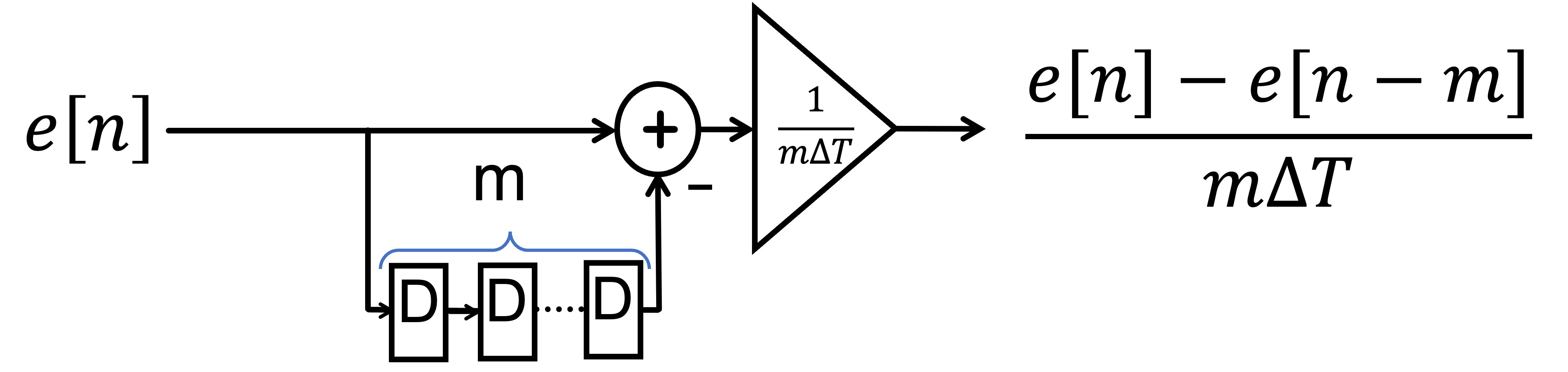
where
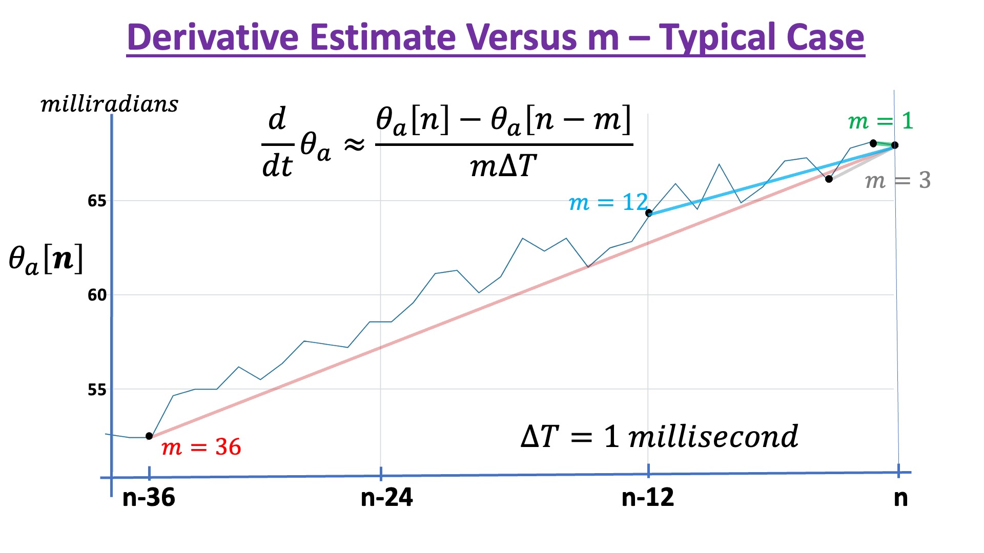
Try increasing m (integers between 1 and 10) using index 0 (EXTRABACK) in the send window. You should be able to set m to produce a figure like the one below.
Simple Model, Simple Control
In this section, we assume that the motor command and arm acceleration are related by a scaling factor, and use that model to determine a second-order difference equation model for propeller arm system with proportional control.
The Structural and Functional Blocks
The main structural components of our angle control system are blocked out below.
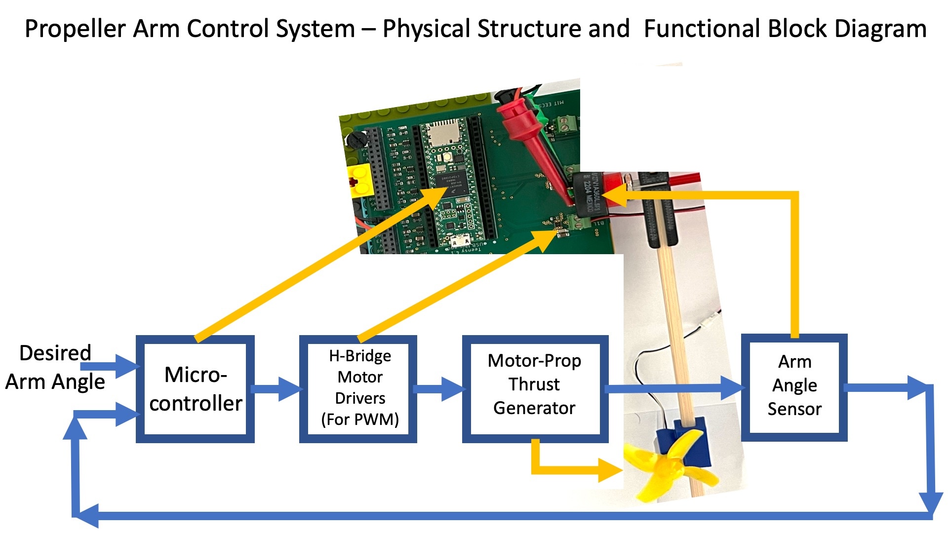
The connection between the structural components and the abstract control functions are detailed in the figure below.
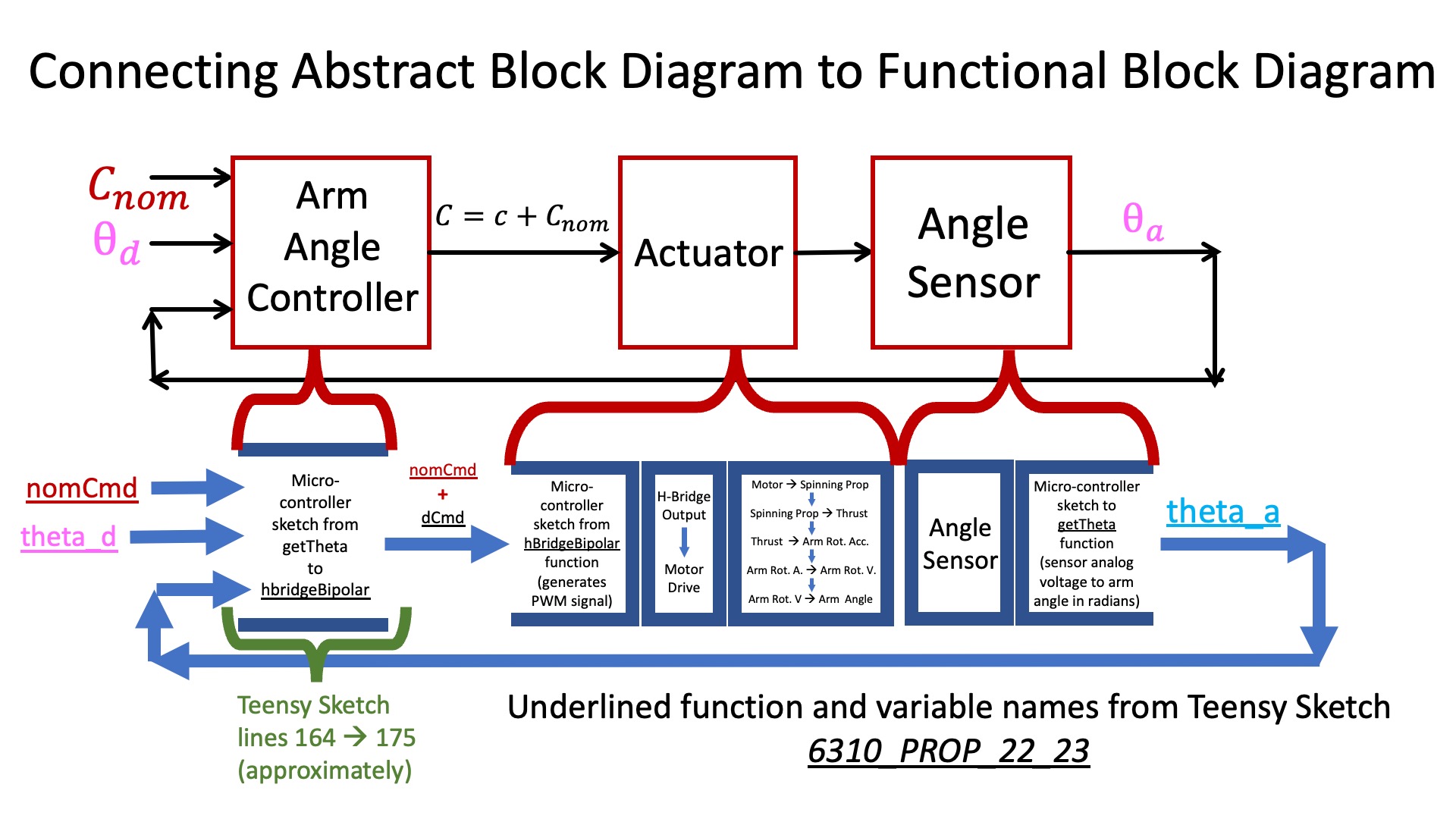
In the above diagram, the command to the actuator (the motor command) is divided into two parts, C = C_{nom} + c. Note that C_{nom} was set to a fixed value during calibration, one that produced a thrust that exactly cancelled any torques due to gravity when \theta_a = 0 (the horizontal arm case). Therefore, as long as we consider small rotations from horizontal, we can ignore C_{nom} and gravity, and develop models that relate arm acceleration to c alone (note "little c").
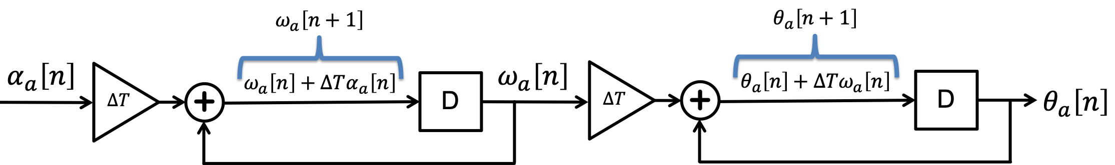
From angular acceleration to angle
Before diving into the deep end (the deep end being modeling the relation between motor command and arm acceleration), let us consider the relationship between acceleration and velocity, followed by the relationship between velocity and angle.
Just like linear acceleration, if the angular acceleration is a constant, \alpha_a[n-1], for the time between the n-1^{th} and the n^{th} sample, then the change in angular velocity, \omega_a, is given by
Or in block diagram form,
A simple model relating motor command to arm acceleration
As we noted above, if the c part of the motor command is non-zero, then the propeller will produce a thrust that is not entirely cancelled by gravity, and that excess thrust will accelerate the arm. So perhaps we can model the relationship between c and \alpha_a as
If we examine the description of the actuator in section 4.1, we can see that we are using a scalar to model a complicated process. That process starts with a change in motor command that gets converted to a change in a motor-driving H-bridge-buffered PWM signal, which in turn changes the speed of a thrust-generating propeller, resulting in a change in arm acceleration. Seems like a lot to expect from one number. And in addition, we already know that there is a non-instant relation between motor command and propeller speed, because we modeled that as part of the first lab.
So, this simple model won't be perfect, models never are, but some are useful. Let us see if this one is.
Proportional Control
By proportional control, we mean that
For the case of proportional feedback control, the system diagram is as shown below.
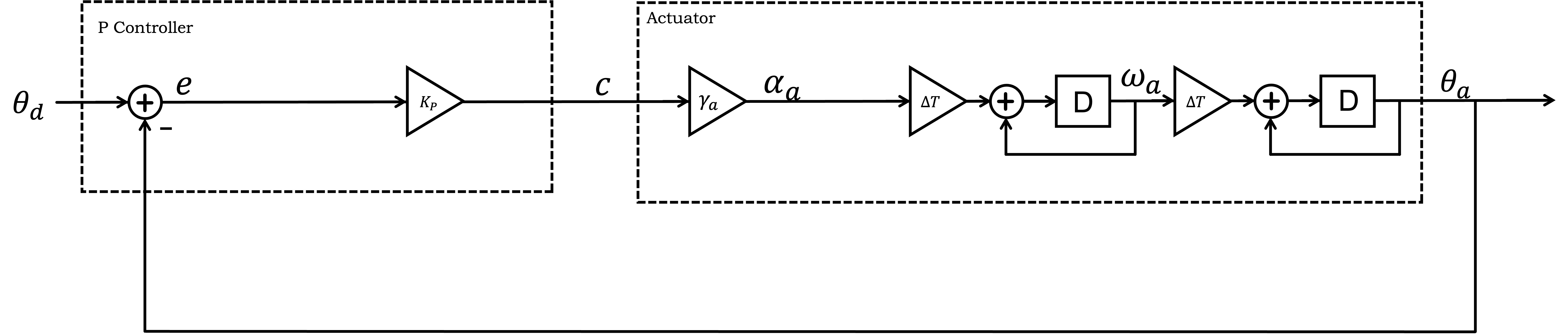
Checkoff 3
Determine an analytic formula for the natural frequencies of the 2nd-order difference equation describing the proportional feedback system above, as a function of \gamma_a and K_p, and then plot them as a root locus in the complex plane. What can you say about the plot, and the stability of the system, without knowing precise values for \gamma_a and K_p?
In Checkoff 2, you found the smallest K_p gain for which your arm produced a growing oscillations when started with a 60 milliradian offset from level. Redo your experiment for the K_p you found before, and then repeat it using twice that K_p. During each experiment, be sure to pause the serial plotter quickly, so you can measure the oscillation periods (using the plotter's curser) when the growing oscillation amplitude is still small. Keep in mind that \Delta T = 0.001 seconds, and that the plotter plots every tenth sample (so there are one hundred plotted points per second).
By comparing these measured oscillation periods to your natural frequency formulas, you should be able estimate \gamma_a for your model, as well as test its prediction (it may be useful to review sections 4 and 5 of oscillating prelab.).
STOP HERE FOR WEEK A!!!!
PD Control
Physical analogies can be misleading when first learning about feedback control, but in the case of the propeller arm with PD control, perhaps the intuitive insight is worth the risk. So, consider the above proportional control experiments on the arm. After you set a gain, you pull on the arm, then let go and then watch the arm oscillate. That sounds a lot like pulling on a spring, then letting it go, and watching it oscillate. Also, spring forces are typically proportional to displacement from equilibrium, with stiffer springs generating larger forces. Analogously, proportional feedback produces a "force" for the arm is proportional to the error in angular position, with larger values of K_p generating larger "forces". So isn't using a larger K_p like switching to a stiffer spring, don't they both result in faster oscillations?
Pull on a spring, and at least in this reality, its oscillation will not grow in time. That is, springs don't go unstable but our arm does. Nevertheless, if one sticks with the spring analogy, then one might be tempted to try "damping" the spring's oscillations by adding a friction term. Friction forces are typically proportion to velocity, the time derivative of position, so perhaps it is not so surprising that one can "damp out" the arm's oscillation by adding a feedback term that is proportional to the position error's time derivative.
We can stabilize our propeller arm by adding a feedback term that is proportional to error differences, and since these differences are usually scaled by \Delta T, we can think of them as an approximation to derivative feedback.
PD Difference equation
We define the error in angular position for the arm as
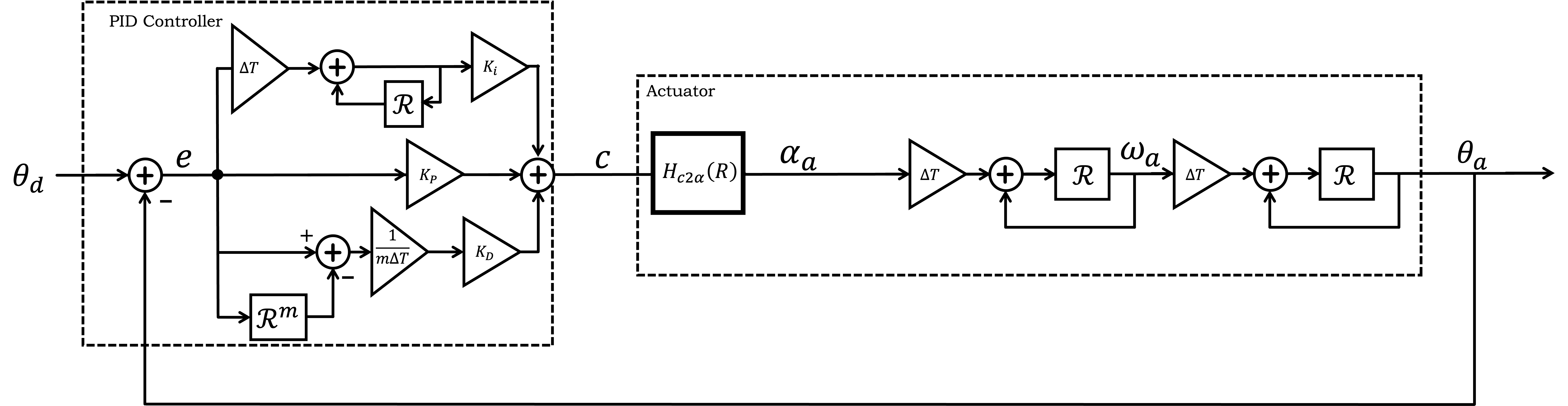
A block diagram for the PD controller, along with our simple second-order actuator model, is give below.
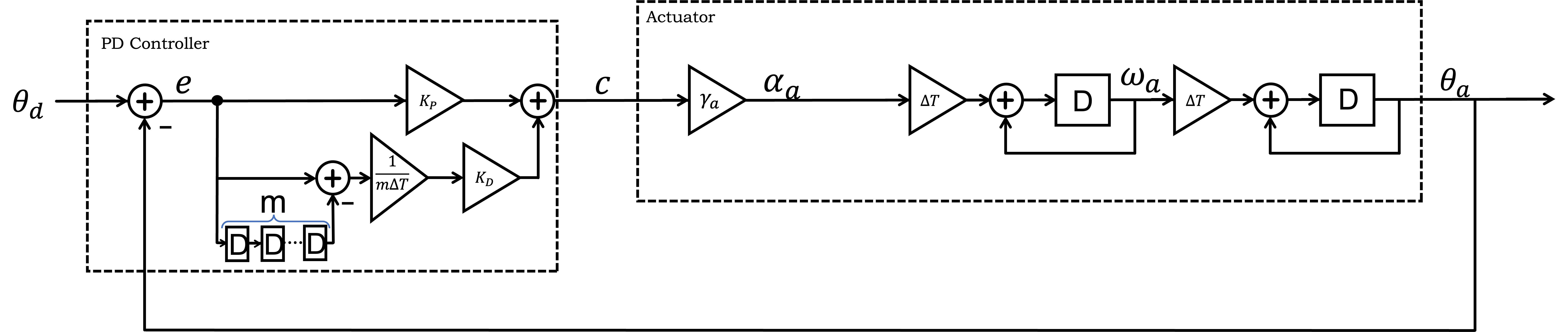
System Difference Equation
The difference equation relating \theta_d[n] to \theta_a[n] is a bit complicated to derive without the operator methods (covered later in this lab), it is given by
Notice that m \ge 1, so the above difference equation is AT LEAST third-order, so finding its natural frequencies means finding the roots of a cubic, or higher order, polynomial.
How many natural frequencies are there for the LDE that describes PD feedback for m=5?
Transfer Function Modeling
Using transfer functions is simple to explain, but not so simple to execute. Multiplying transfer functions described by rational functions in R means forming products of polynomials, a task best left to a computer. There are lots of computational tools for manipulating transfer functions, and we provide matlab scripts as a template. We also know that many of you are writing your own tools, using python or Julia, which we strongly encourage and applaud!
Matlab Model
The diagram for the PD-controlled propeller arm model, with the simple model relating motor command to arm angular acceleration, is repeated below with R and powers of R used to represent delays.
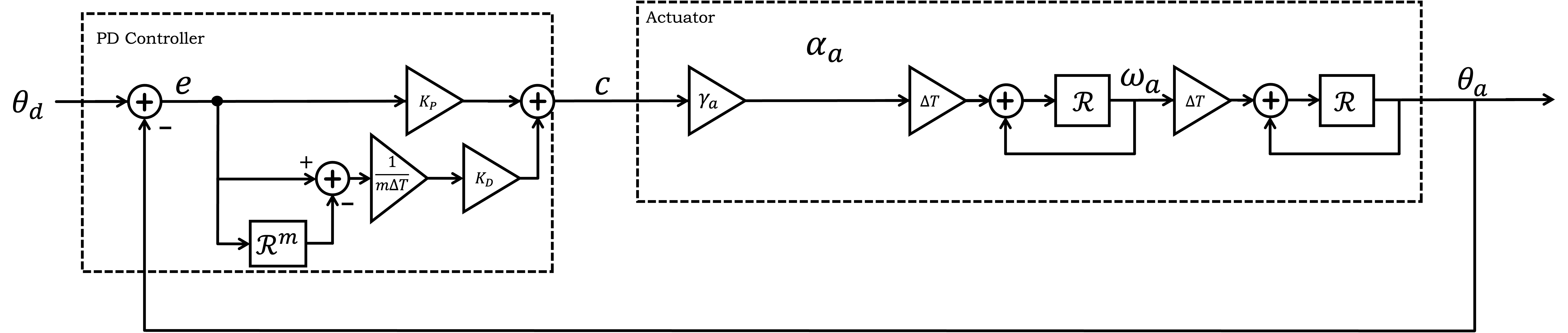
We have provided a matlab script, rootPlotLab02.m, for analyzing linear models of the propeller arm system. The script generates a plot of the loci of natural frequencies for specified ranges of feedback gains, and also plots two step responses associated with gains at the lowest and highest ends of the range. In the script, the difference equations associated with the above block diagram are represented using rational functions of the delay operator R (a first-principles alternative to a z-transform framework, one that generates equivalent analyses when z^{-1} is substituted for R).
Matlab Model Organization
In our matlab script, we created transfer functions to model each section of the above diagram: the Teensy controller, Kpid, the Teensy motor command to arm acceleration, Hc2a, the arm rotational acceleration to rotational velocity, Ha2w, and the rotational velocity to arm angle, Hw2t. Note that in the matlab file, the transfer function from motor command to arm rotational acceleration, Hc2a, uses the instant model, so is specified as a single scale factor, \gamma_a. And the Kpid transfer function is missing the implement of the integral controller.
As you can see in the matlab script, we then created transfer functionals using R. For example, we created 'Hw2t', the transfer functional from arm angular velocity \omega_a to arm angle, \theta_a. Recall we have a difference equation relating \theta_a to \omega_a,
The system functional relating \Omega_a to \Theta_a is then
In the matlab script, we write the system functionals and let matlab convert to system functions, as in
>> Hw2t = dT*R/(1-R).
where we define R = z^{-1}. Below is a summary of the system functionals:
- `Hw2t`: rotational velocity to arm angle,
- `Ha2w`: arm acceleration to angular velocity,
- `Hc2a`: motor command to arm angular acceleration (Needs fixing),
- `Hc2t`: the complete open loop model without the pole (just the product of the others!!).
- `Kpid`: The PID controller transfer function (Needs fixing).
We derive the transfer functional as ratios of polynomials in the delay operator R, and matlab converts them into system functions by substituting R = z^{-1}. But matlab also tries to eliminate the negative powers of z, effectively multipling the system function by \frac{z^k}{z^k} for some k. If you are converting rational functions back into difference equations, it is important for the numerator and denominator to be polynomials in R, or equivalently in matlab, negative powers of z. But if you are calculating natural frequencies (or equivalently poles), by determining the roots of the system function's denominator polynomial, then the effect of matlab's conversion is to add extra poles (cancelled by "zeros", the roots of the numerator polynomial) at \lambda = 0, which you can safely ignore.
You can either write your own version of our script in the language of your choosing (lots of students are making excellent use of jupiter notebooks, and we'd love to see any Julia implementations). Regardless, you will be adding to our script or your own version, both to include a better arm model and to add the sum (or integral) term to the controller.
Testing the Matlab Script
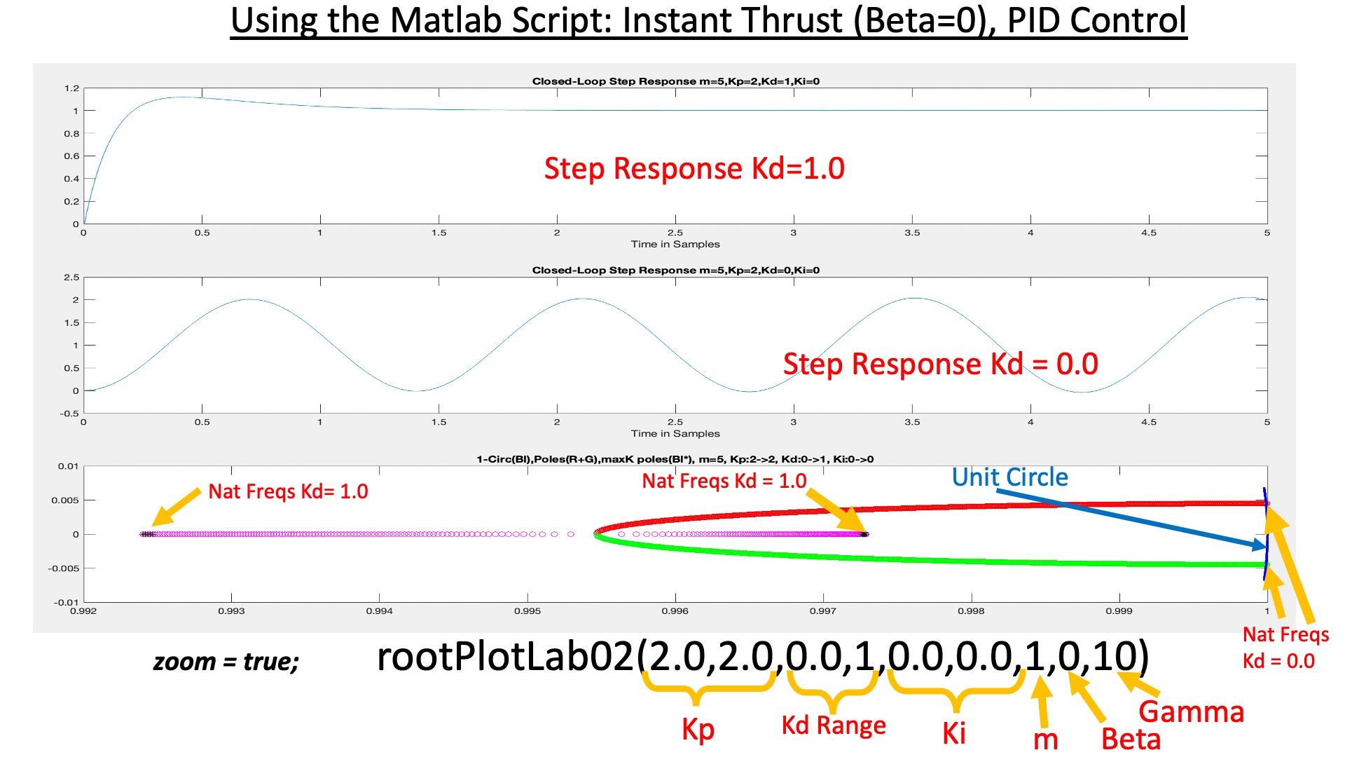
Try running the matlab script with the command below, and see that it produces an array of three plots, two step responses and a root-locus of the closed-loop system natural frequencies (or poles) as K_d ranges from 0 to 1. The plotted step responses are associated with the K_d=1 and the K_d=0 values. In general, the step responses are plotted for the minimum and maximum values for the gains over the given ranges.
The command below generates pole plots from the system model (with m=1, \beta = 0, and \gamma = 10), with K_p = 2, K_i = 0, and K_d varying from zero to one.
rootPlotLab02(2.0,2.0,0.0,1,0.0,0.0,1,0,10)
You can examine how the poles (natural frequencies) change with parameters (in the case, K_p=2 and K_d ranges from zero to one). Note that we have marked the poles associated with the highest values of K_d with black stars inside circles (see the figure below).
Revisit PD Control
The matlab script implements the simple motor command to acceleration model, the same one you calibrated above using oscillation periods of the destabilized arm. Also, please revist the step response cases examined in section 4.6 above
Try the following and compare the matlab step responses to your experiments. Please keep in mind that you will have to scale your experimental results when comparing to matlab step responses.
- Set K_d = 0.1 (type "1 0.1" in the send window) and K_p = 0.5
- Set the step frequency to 0.2 (type "5 0.2" in send window), and then set the step amplitude. First set the amplitude to 0.05 (type "6 0.05"), then to 0.1, and then 0.2.
- Repeat steps 2-4 with K_p = 1.0, and then 1.5, and then 2.0. Does the arm go unstable? Are the natural frequencies of your third order model above consistent with that instability (you can use matlab's roots command to compute a few roots)?
Show a screenshot when the propeller arm was stable.
Show a screenshot when the propeller arm was unstable.
What does the Matlab script predict in each of these cases?
Be prepared to explain these results.
Better Controls, Models, and Manipulations
PID (Proportional, Integral, Derivative) controllers are ubiquitous in feedback systems, though for discrete-time systems, it would be more accurate to refer to such controllers as PSD (Proportional, Sum, Delta). An ad-hoc approach to designing a PSD controller is to select a proportional feedback gain, K_p, and then increase the gain of the Delta (or derivative) feedback, K_d, until the step response is sufficiently stable. Finally, add Sum (or integral) feedback, with gain K_i, to eliminate any remaining steady-state error.
So if we can easily run experiments, even automate the running of those experiments, what is the value of modeling? With a model we can get far more information that just the result of a single input-output experiment. In particular, we can compute the closed-loop system's natural frequencies as a function of PID controller gains, K_p, K_d, and K_i,, which will tell us how the system will response to a whole of range of inputs and disturbances. In addition, we can even generate plots of how those poles (another name for natural frequencies) move as a function of a parameter, a generalization of the so-called "root-locus" plot. Such plots can tell us what is feasible, like when we used a plot of poles versus proportional gain above to show it was impossible to stabilize the arm with proportional gain alone. Finally, we can use the model to solve a minimax problem with respect to the magnitude of the poles. That is, we could let the computer search through millions of senarios, to find the gains that minimize the closed-loop system's maximum magnitude pole. We would then be sure that resulting closed-loop system would be fast, and that any errors would decrease rapidly. But we digress. There is much to the story of data and models, some of it with connections to machine learning, and this issue will reemerge many times during the semester.
Back to the matter of finding a good model. Above, we calibrated a model of the propeller arm based on assuming the arm acceleration was proportional to motor command c. The model was good enough to help us understand some of relationships between controller gains (K_p mostly) and poles (aka natural frequencies), but DID NOT PREDICT THE ONSET OF INSTABILITY when K_d=0.1 and K_p is increased. Seems a pretty serious flaw.
Since we know that propeller thrust does not change instantly with changes in motor command (because thrust is related to propeller speed, and from the speed control lab we know motor speed does not change instantly with changes in motor command). And to further complicate the system, we should also include the sum (integral) term in the controller. So, we have a daunting analysis problem. If we had to rely on the rather cumbersome procedure of shifting indices in difference equations, the task would be unbearably tedious. Instead, we use the delay operator, R, to convert those shifts into multiplication by powers of R, and to convert difference equations into ratios of polynomials in R. These ratios of polynomials, rational functions, are also referred to as transfer functions, because when we compose systems described by difference equations, we can just multiply their associated transfer functions.
Non-Instant Motor Command to Arm Acceleration Model
Propeller thrust produces arm acceleration, and thrust tracks propeller speed instantly but nonlinearly, being approximately proportional to the square of the instantaneous propeller speed. Propeller speed tracks motor command, but not instantly, and somewhat nonlinearly. Together these observations might suggest we need a very non-linear and non-instant model relating motor command to arm acceleration, but that is not the case. The motor command to arm acceleration is suprisingly linear (fortuitous cancellations no doubt), though definitely NOT instant.
Above we used oscillation period measurements versus proportional control gain (K_p) to calibrate \gamma_a in the following relationship between motor command and arm acceleration,
If c[n] = c[\infty], a constant, and -\frac{1}{T} < \beta < 0 , then what is \lim_{n \rightarrow \infty} \alpha_a[n]?
Testing the PD controller and the model.
Implement the above non-instant model in the matlab script, and calibrate the values of \gamma_a and \beta by matching the computed step responses to measured steps on the arm for various values of K_p and K_d. Keep in mind that the matlab model is linear, so keep your step sizes small (e.g. "6 0.05"), Also, it is easier to match waveforms that are highly oscillatory waverforms. Save screenshots of step response in experiments and simulaton with the same set of control paramters.
Sum (Integral) Feedback
We can add an integral, or more precisely, a sum feedback term to our controller. The advantage of including an integral term is that any persistent error, no matter how small, will cause the sum to grow steadily. When the sum term is large enough, it will cause an adjustment to the motor command, persumably an adjustment that eliminates the small error.
The motor command with the proportional, delta, and sum feedback can be described by the difference equations
Testing the PID Controller.
In this section you will analyze our new closed loop system and conduct experiments to understand the model's predictive power.
- Add the integral term to the matlab model for the controller, Ki.
- Use your complete matlab model to design the gains of your controller. What are you going to try to minimize? Note: There are practical tradeoffs to make here. The higher the gains, the more the noise in measurement will effect the output. The lower the proportional gain (and associated K_d), the slower the response and greater the error. This choice is an open ended question. There is no 'correct' answer, but rather, many answers can be justified. You may have to try several sets of values to zero in on a good solution. Use computation and your model!!
- What does your linear model tell you about steady-state errors with and without the integral (aka sum) term? To see the advantage of using the integral term, try dropping a Lego "U" on the arm as shown in the picture below.
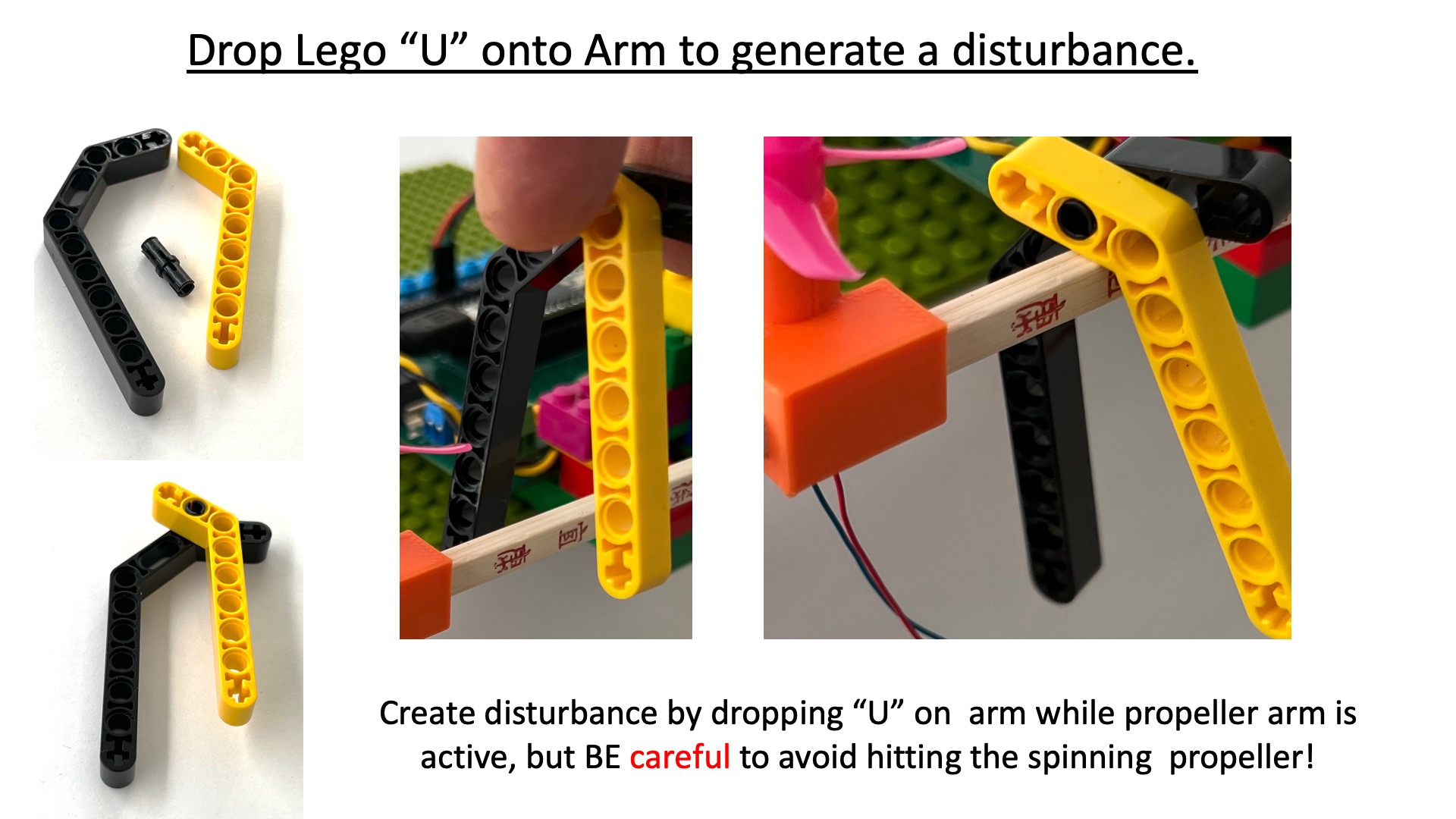
How does the predicted behavior for your system (examine the calculated poles and plots of step responses) compare to the experimental behavior with large (>0.3) input steps. Try dropping a Lego "U" on the arm, how does the response change with a zero and non-zero K_i. Does K_i > 0 improve disturbance rejection? Find values of K_d, K_p and K_i so that the step response is reasonable and you get some "dropping Lego U" disturbance rejection.
Explain how you tuned your values of K_p, K_d, and K_i. To analyze the response to disturbances, a disturbance transfer function is needed, a topic we will address that in the postlab. TAKE SCREEN SHOTS OF YOUR DROPPING THE LEGO U EXPERIMENT WITH ZERO AND NONZERO K_i, to use for your postlab.